Building a Simple Plagiarism Detector
Sep 03, 2022
Wherein I build a simple plagiarism detector and compare a couple different word embedding models against each other.
All right, I’m going to start out with a literature review, by just jumping on Google Scholar. Bam! Here’s one:
arxiv.org/pdf/1801.06323…
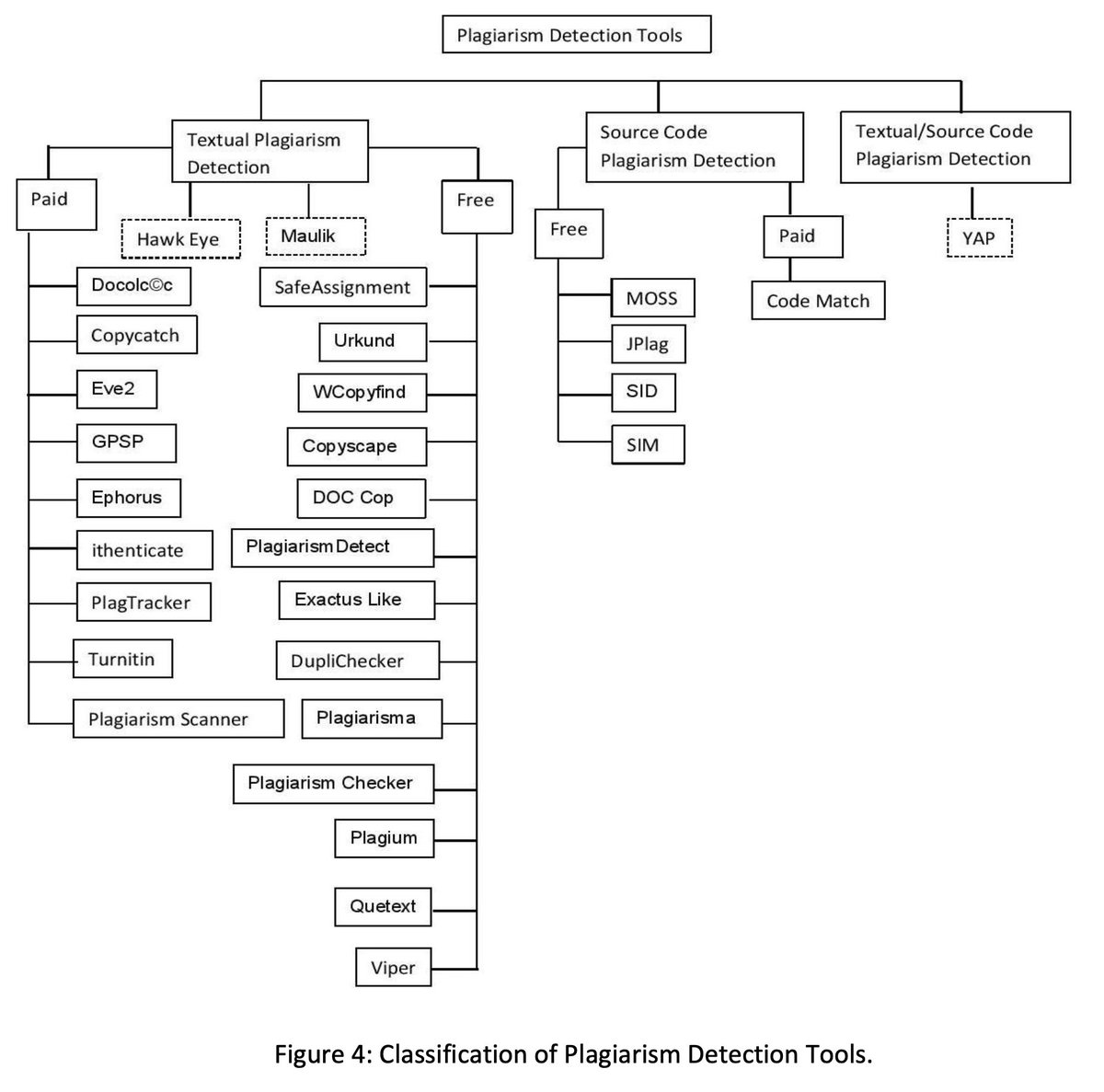
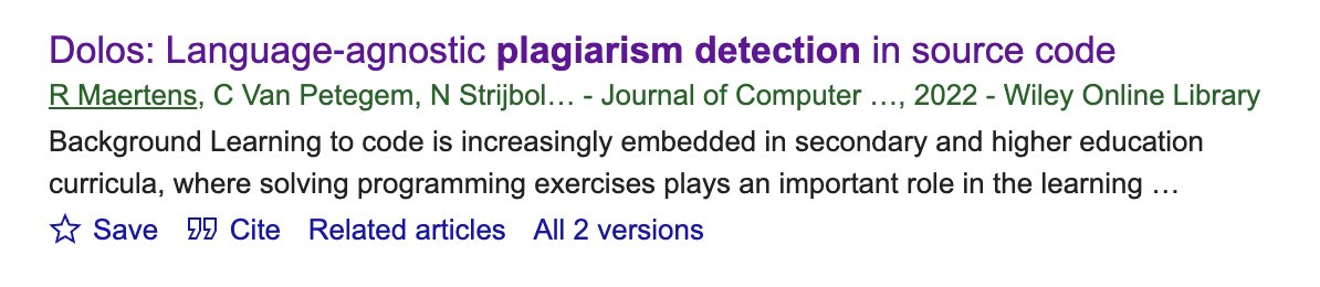
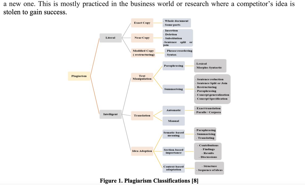
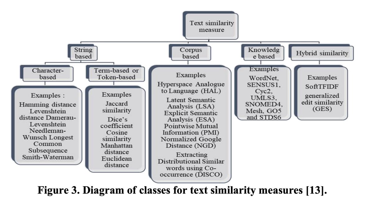
Chowdhury and Bhattacharyya break down a taxonomy of plagiarism, presumably from a review of literature, since the study is cited as a survey. They also mention cross-lingual plagiarism, a clever little way of simply translating ideas from one language to another.

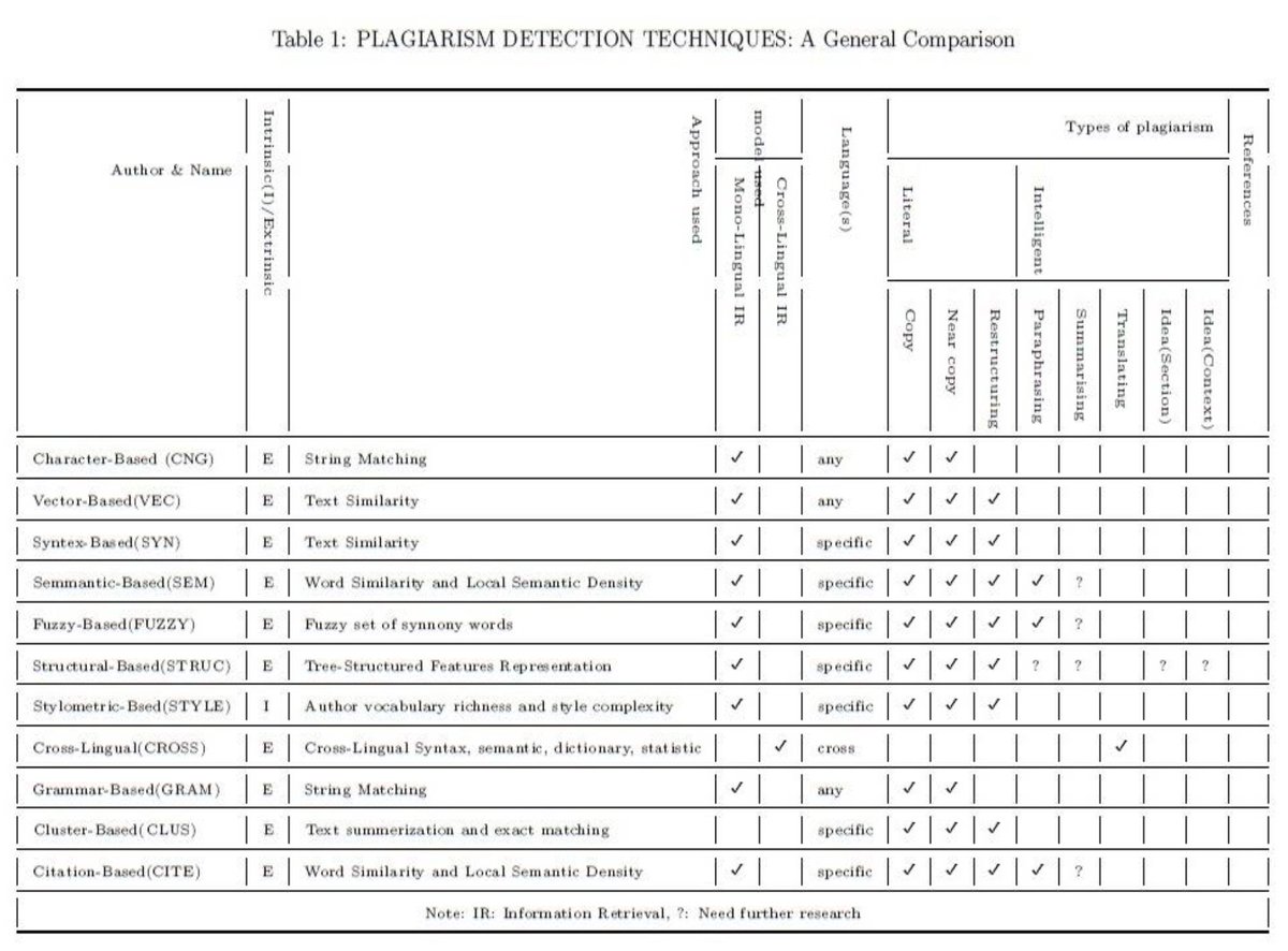
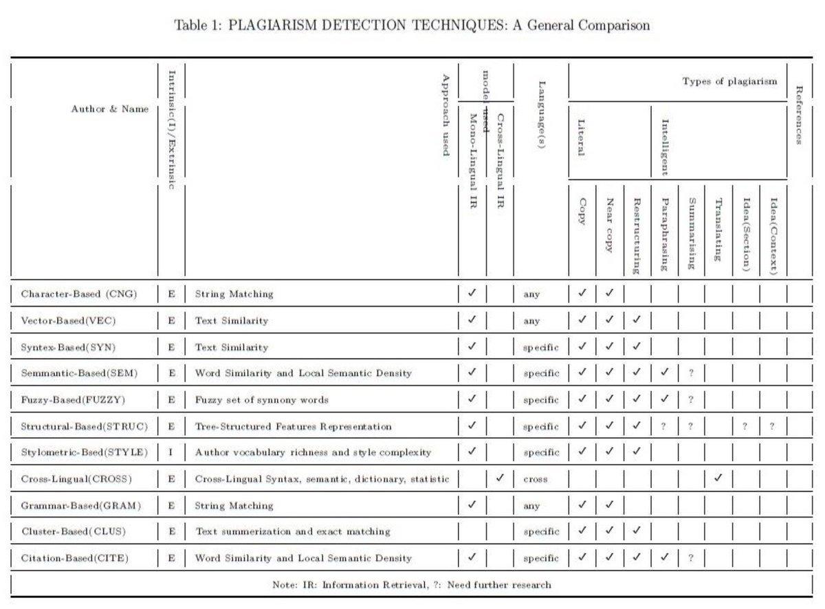
Chowdhury and Bhattacharyya identify 11 different techniques for plagiarism detection developed over the previous decade and summarize them all in a table.
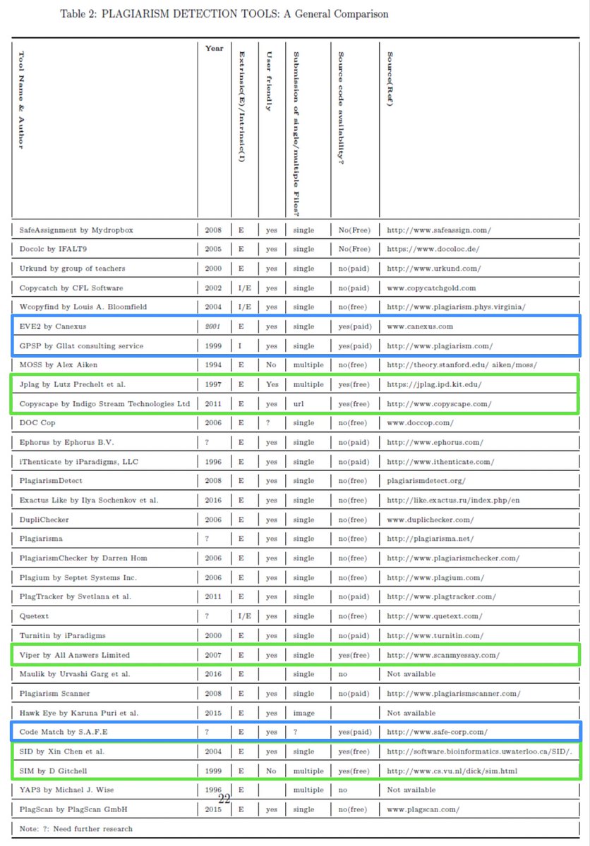
Chowdhury and Bhattacharyya also identify and summarize 31 different plagiarism detection tools, which includes 5 free and open source tools, as well as 3 paid open source tools.
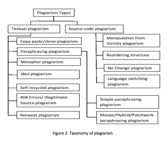
…there was also a distinction made between “Textual Plagiarism Detection,” as well as, “Source Code Plagiarism Detection.” So interestingly, the world of plagiarism detection is not only concerned with academic/textual work but also source code.
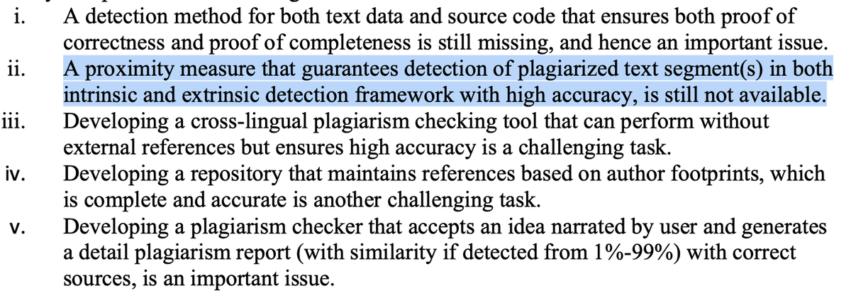
The paper concludes by listing some challenges in plagiarism detection, as well as the notion that no guaranteed detection method exists. They also pose an interesting idea, the concept of a real-time idea checker, which shows an author whether their idea is original or not.
Looking further into Google Scholar:
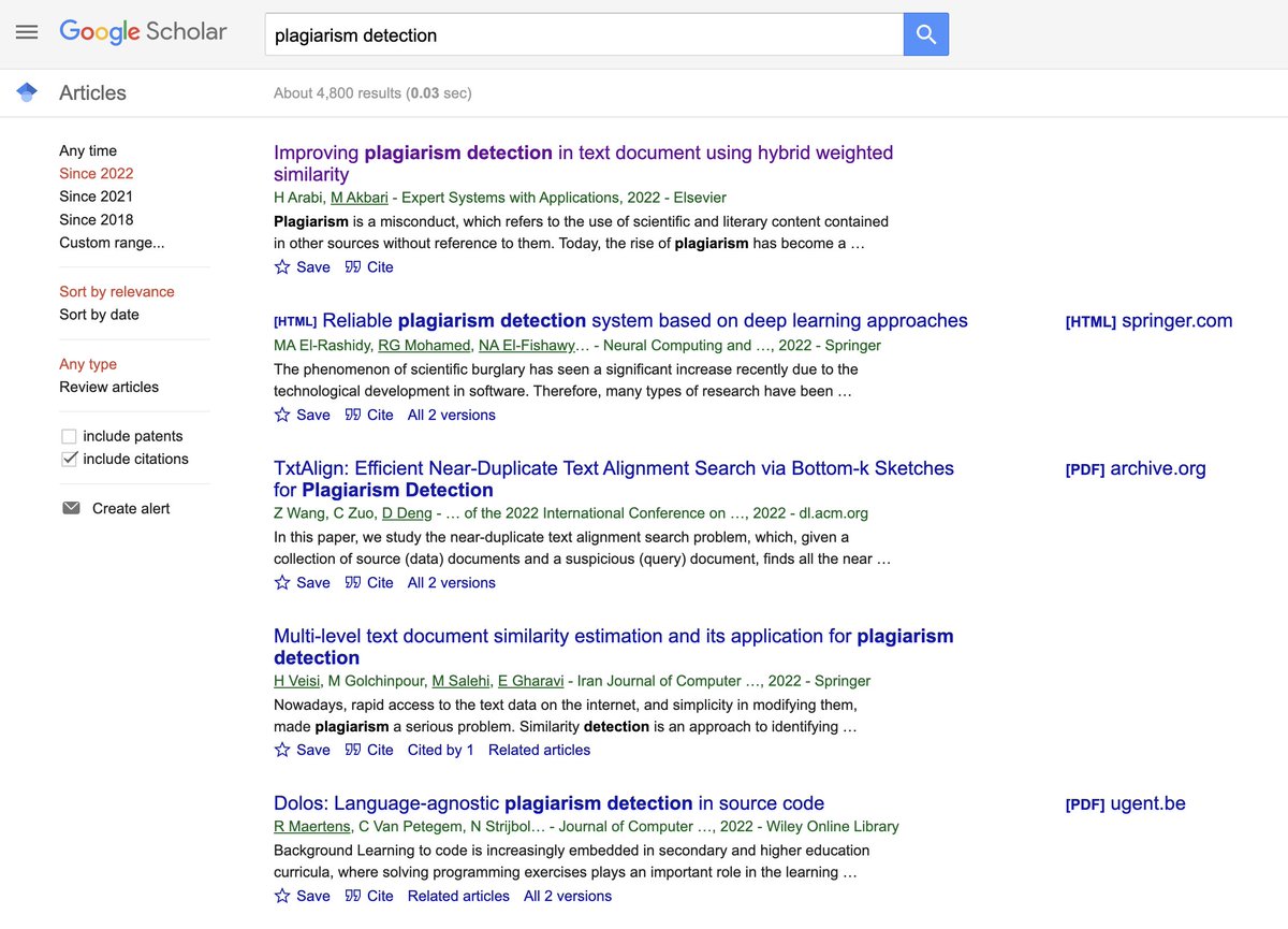
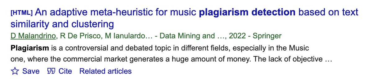
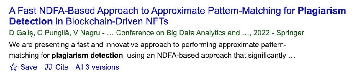
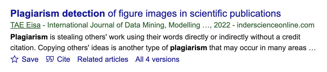
While breezing through Google Scholar for plagiarism detection, I found papers on: music, source code, more surveys, NFT’s, images in scientific publications faculty attitudes on … almost 5000 results in 2022.
The paper on faculty attitudes toward plagiarism detection is interesting, it basically reads like an advertisement for something called Ithenticate.
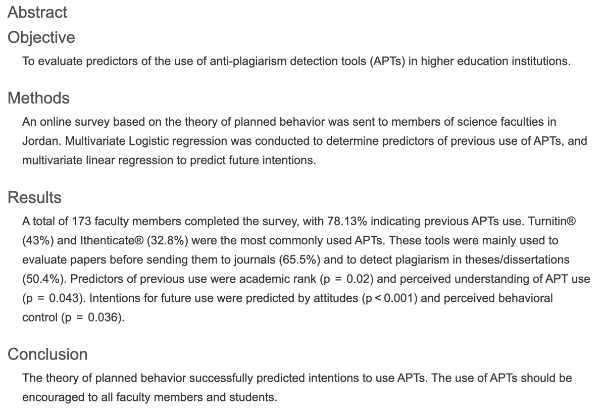

Ithenticate charges about $0.004 USD per word on bulk text, with evidently no break if you buy multiple, but they will certainly sell multiple to you! 😂

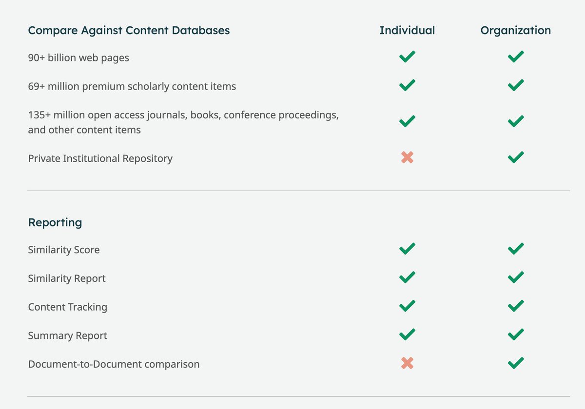
Ithenticate provides two tiers of service - they use a database of 90+ billion web pages, and a bunch of articles, journals, books, conference proceedings, etc. They provide a similarity score, report, and summary and something called, “Document to Document Comparison.”
This seems similar to another service I had found the other day called, “Unicheck,” which charges $0.06 per page rather than $0.04 per word. Unicheck seems to highlight usability and integrations rather than a vast database.


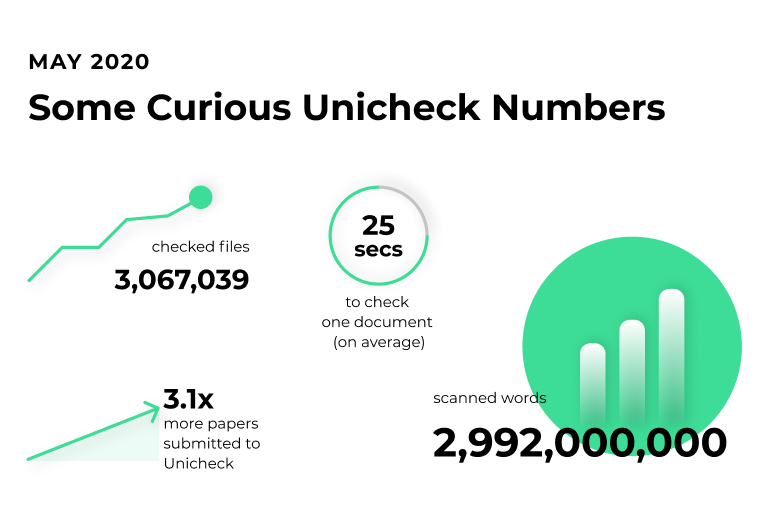
Unicheck on their social media claims to have scanned as of May 2020, about 3 billion words. So assuming they were being sneaky and that this actually represents their training database, not their customers, and assuming 4k words/paper, they have a database of around 750k papers.
I find this whole area interesting, because to me these seem like tools geared toward beating other plagiarism detection services or rather, beating humans at their ability to detect plagiarism. So rather than policing plagiarism, they are enabling more sophisticated plagiarism.
Basically what I’m saying is, these seem like tools to help someone game academia. The extension of this thought is that this could become a scenario where increasingly powerful tools are used on both the policing side and the, “hint making,” side in an escalating conflict.
But anyway, here’s another open paper I found surveying plagiarism detection approaches, this one from a University in Iraq.
edusj.mosuljournals.com/article_170205…
Interestingly this paper by Taqa and Ali breaks down plagiarism into, “Literal” and “Intelligent” detection methods, which differs from the survey above by Chowdhury and Bhattacharyya (I’m becoming hyper aware of whether one of these papers may have plagiarized the other).
At the end of the day, both of these surveys point toward the notion that more recent plagiarism detection methods seem to work based upon some kind of similarity or distance metric, with the former survey also citing string matching.
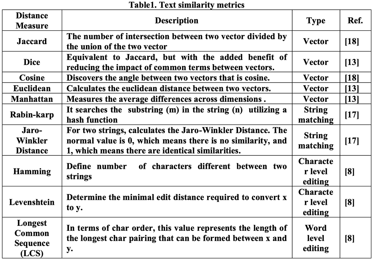
The way I visualize these methods in my head is the following: string matching is essentially looking for an exact string, “abc 123,” : if two texts contain the same string, one may have plagiarized the other. This is a much more, “direct” way and assumes direct copying.
Similarity or distance matching, is on a basic level, like calculating pythagorean distance, but rather than calculating the distance (c) with two dimensions, you calculate it with many dimensions.
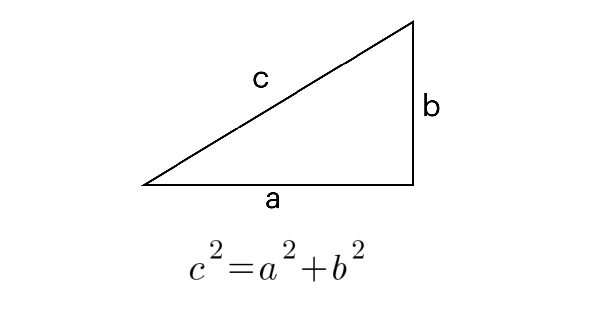
Rather than physical or linear distance using two or three dimensions, we match multiple, hundreds or thousands of dimensions using tokenization, where a token represents a word, sentence fragment, or phrase assigned a code.
If every unique token is given a unique code, one can calculate the distance between series of tokens by treating them as arrays; just like you could calculate the pythagorean distance between [(1,1)(0,0)] you could calculate the distance between two vectors of form (a,b,…n)
The similarity methods discussed in these papers mention many different ways of calculating similarity with underlying algorithms and filters.
So one way to compute textual similarity using open source would be just just follow one of many tutorials online, for example this one from BERT.
sbert.net/docs/usage/sem…
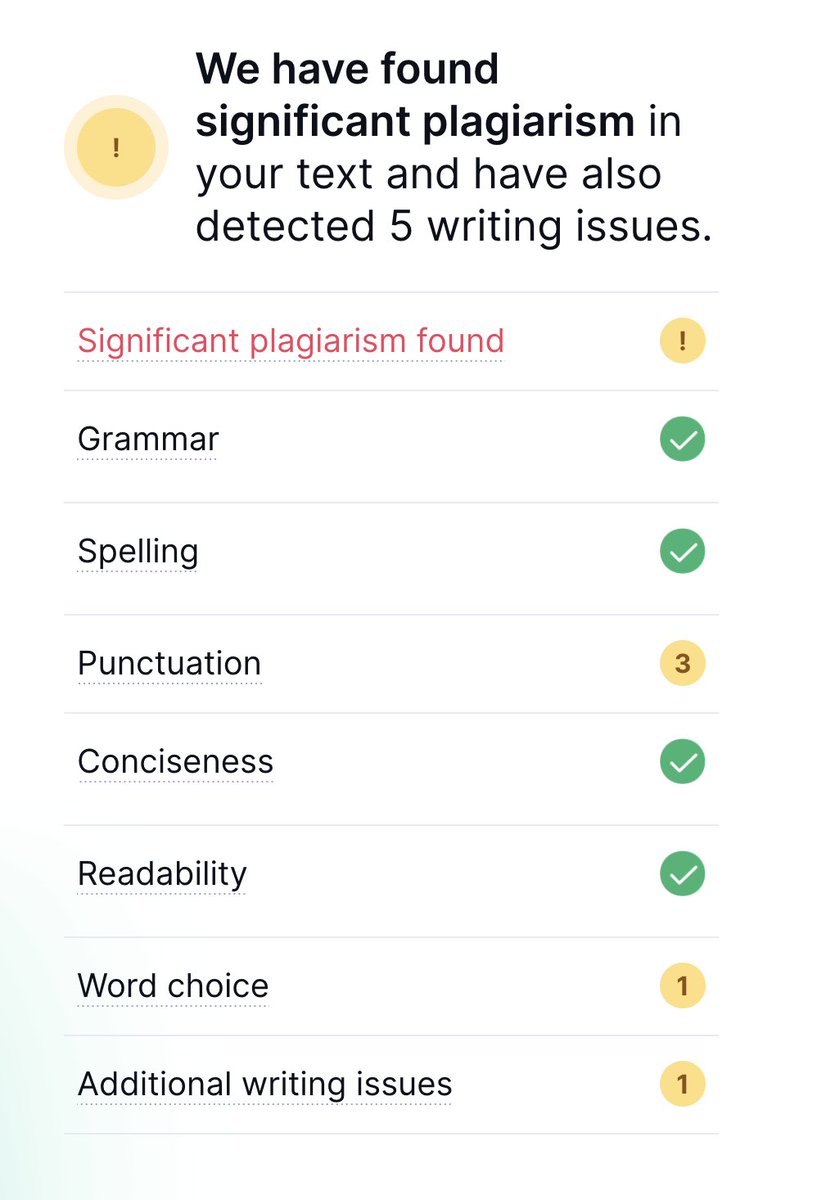
Let’s take a look at what Grammarly does in their free online sample plagiarism checker. Checking some lines from Shakespeare’s Coriolanus, Act IV, Scene 7.

With that above example, which was directly lifted from the text of the play, they of course found significant plagiarism.
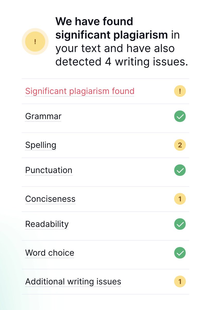
Let’s see what happens if we maintain the idea of the text, but change the wording, which is akin to translation-based plagiarism. We see that the tool also flags our text for plagiarism. Of course this is marketing-focused, so it could simply be hyper-sensitively tuned.

What if we feed in a string of gibberish? Interestingly the output is not only free of plagiarism signals, it’s also free of any grammar, spelling, punctuation and other errors, even though it was completely meaningless text.
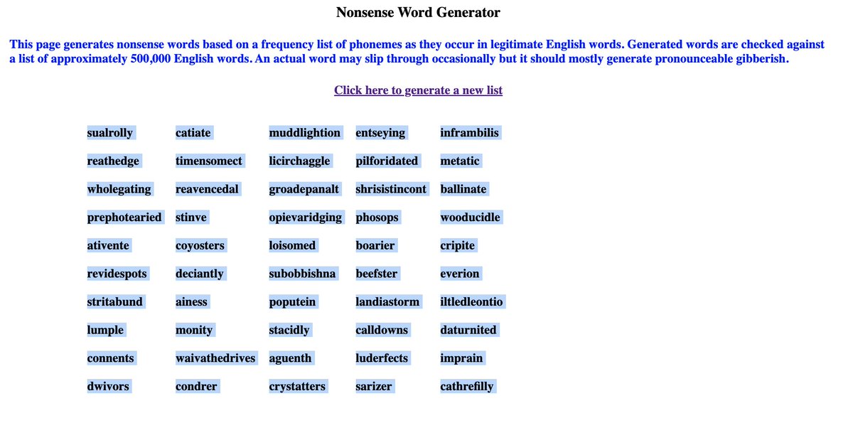
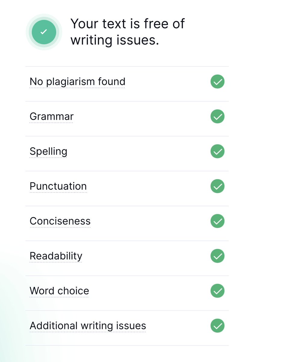
So while this free tool test may not have told us much, it at least showed us that - words which are similar to other paragraphs which may have been written over time are going to measure higher in similarity to a random string of non-existent gibberish words, which is expected.
Ok, so now that we have a very general idea of how plagiarism detection works, we can work toward building a prototype. The first logical step in my mind would be to build something simpler on an existing dataset, perhaps a clustering algorithm on an open dataset.
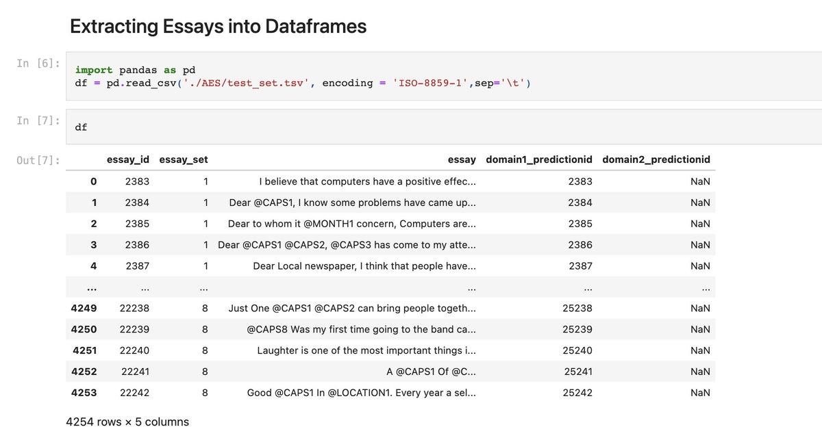
Here’s a collection of various essays written, designed for educational scoring prediction.
ltl-ude.github.io/EduScoringData…
kaggle.com/competitions/a…
Here is the data on Github, so one doesn’t have to sign in to Kaggle (which requires you to provide your phone number for verification for some reason).
github.com/Turanga1/Autom…
And here’s an interesting transformer’s library built for computing sentence similarity.
huggingface.co/tasks/sentence…
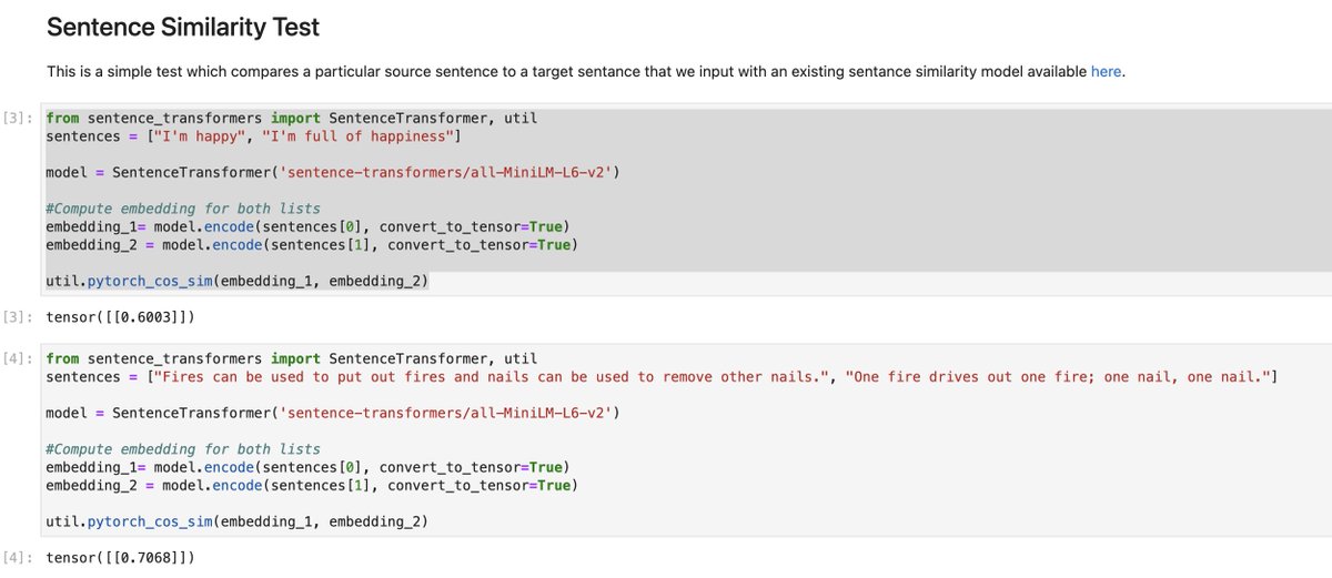
This library even has a widget on the side of the webpage which allows you to compute sentence similarity on the fly.

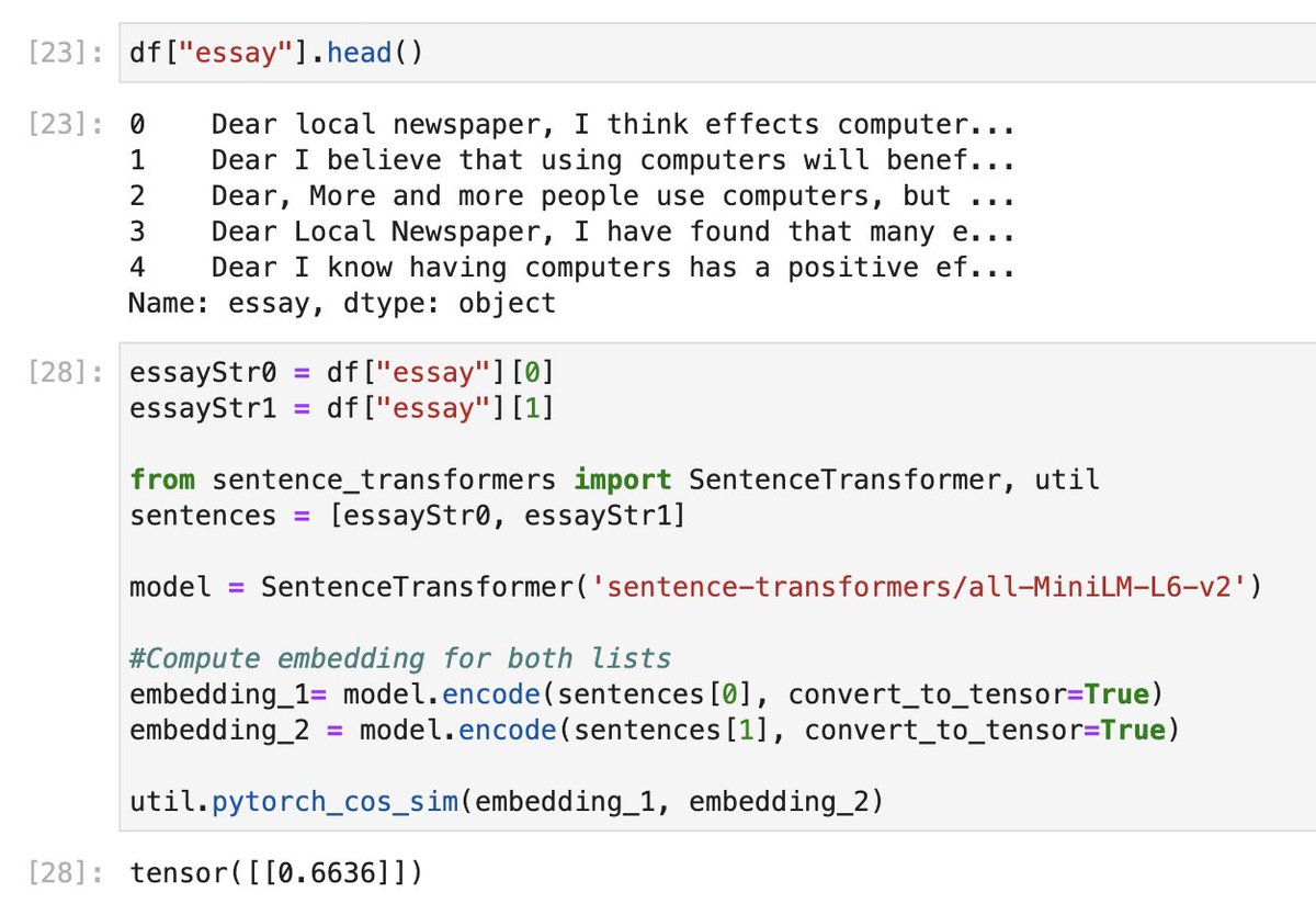
Using a stock example within a Jupyter notebook allows us to compute a sample tensor similarity score between two stock sentences. Using the Shakespearian plagiarism example from above, interestingly we find that the tensor score is even higher than the stock sentence example!
After looking at some of the data up close after putting it into a dataframe using Pandas, I’m realizing that this original dataset has all sorts of weirdness to it which is relevant to data cleaning, e.g. the non-word, “@ CAPS3” and things like that.
So instead of dealing with cleaning, in order to have more of a hacker mentality, I may just use someone else’s already pre-cleaned version of this data sitting in a different Github Repo.
raw.githubusercontent.com/sankalpjain99/…
Looking at this dataset, the, “processed_data.csv” has a few different columns, it looked like the, “clean” data may have been an effort to remove common expressions, as they state in their github, to reduce skewness to simplify the essay grading process.
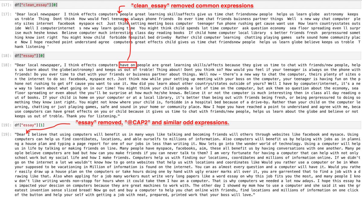
We’re just interested in whatever the closest thing to a human input might be for the time being. Normalization increases computing efficiency, which is an optimization that can be done later. For now, I just want to get a distance measurement between sentences.
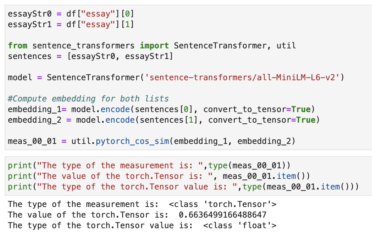
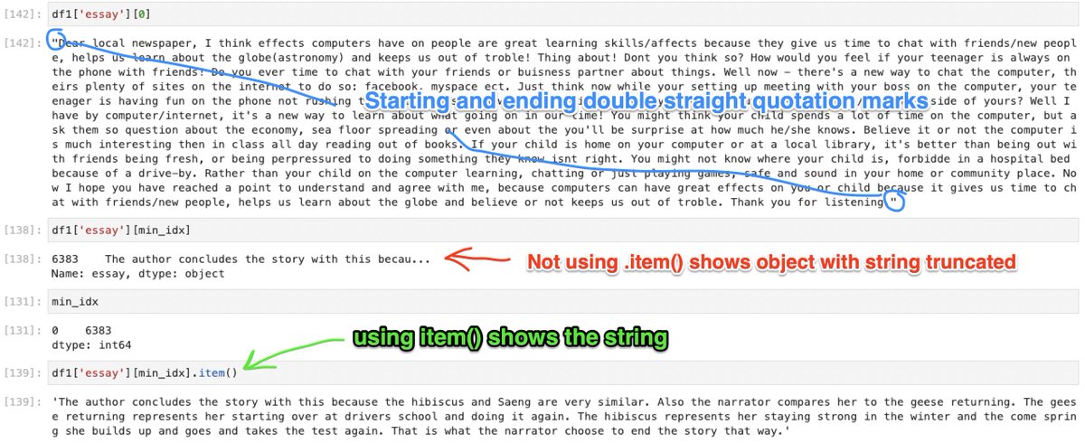
The above output is a tensor, which is a class from Pytorch. We can extract the value with the method .item() as shown below.
pytorch.org/docs/stable/te…
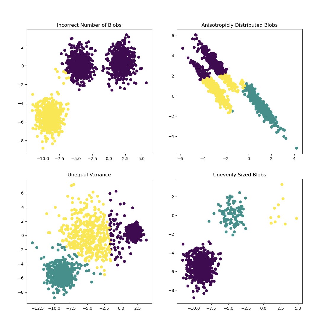
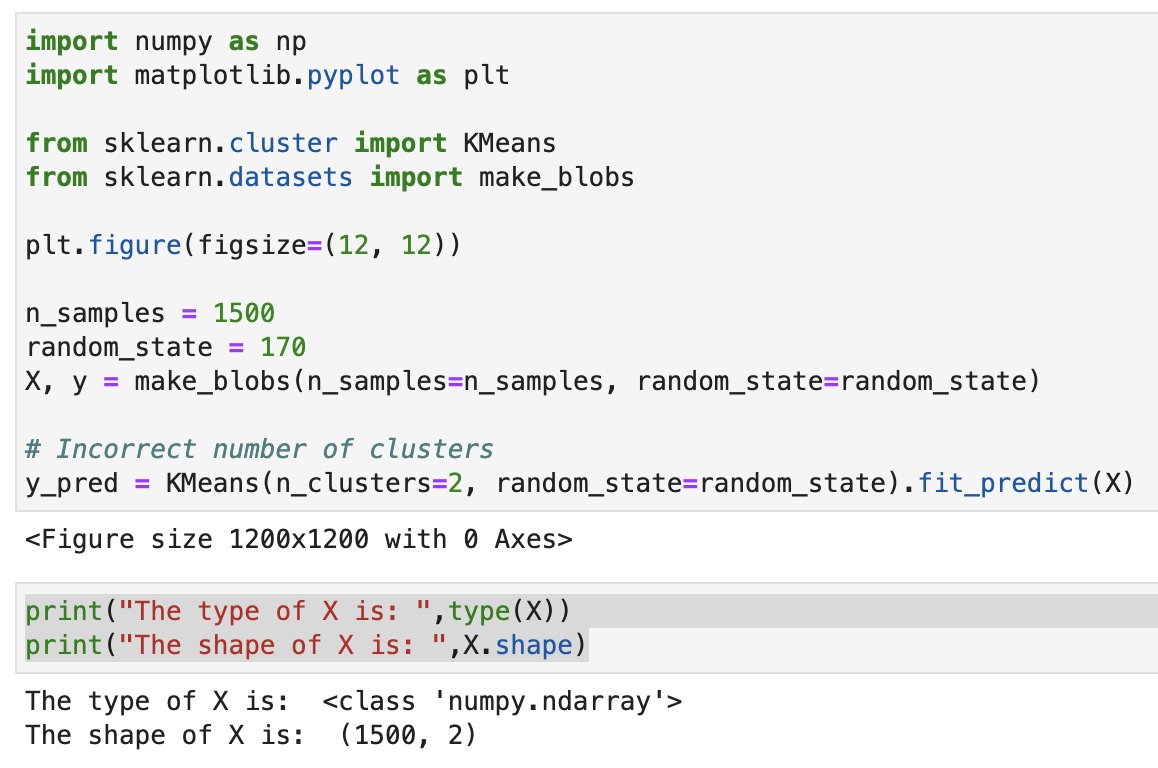
Since we’re able to extract distance between sentences, we can hypothetically do k-means clustering to visualize the various essays against each other. Scikit-Learn has a clustering method, here is a sample:
scikit-learn.org/stable/modules…
If we’re going to do K-means clustering, we have to first reduce the dimensions down. If you look at the dimensions of the input to K-means, you can see that it’s an n*2 matrix, whereas comparing all of our essays together would be a thousands by thousands matrix.
So, one way to do this is with Principle Component Analysis, PCA, which is a way to reduce dimensions (matrix size). A simple way to think about this is we’re setting the objective to create a, “factor,” (eigenvector) that minimizes variance.
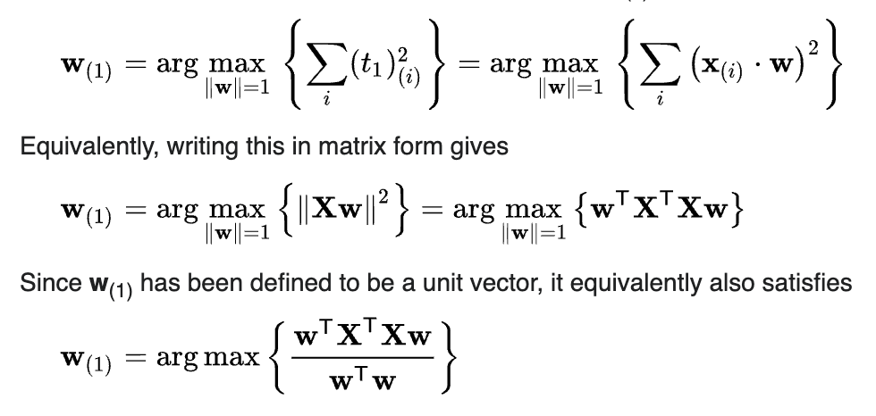
So what that fancy math thing above does is it takes that thousand dimension matrix and grabs the, “most important” part of what makes that matrix special, and distills it down into two (or three, or whatever) dimensions (components), which can be much more easily visualized.
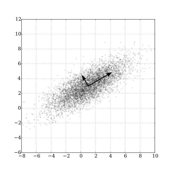
You can probably imagine where we’re going with this. We’re going to take a 2-dimensional graph and then apply another step, cluster analysis onto it, so we can identify essays into groups.
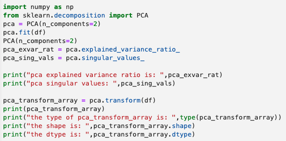
Demonstrating how
pca.fit
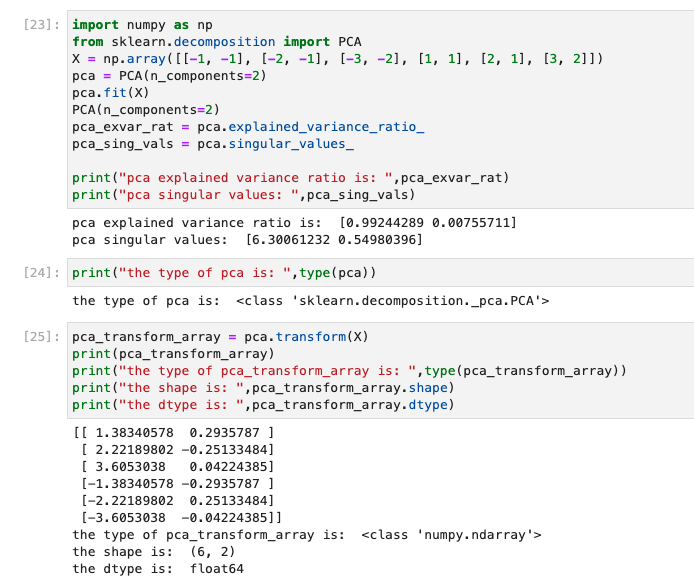
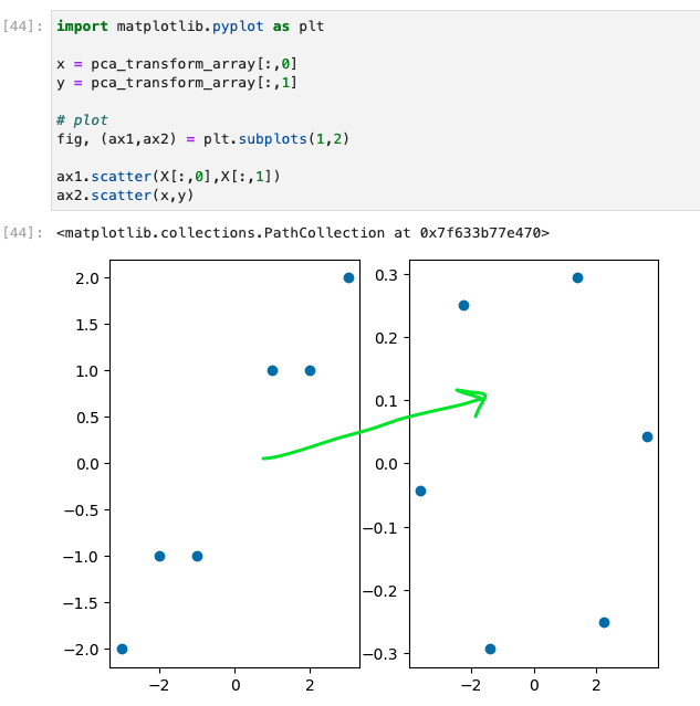
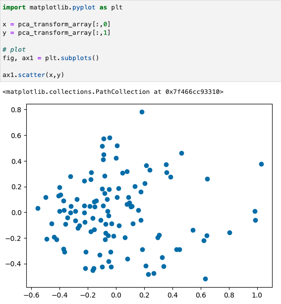
Similarly, we can reduce a 3-dimensional array to a 2-dimensional array with PCA and look at the scatter plot of our original 3-dimensional setup vs. the transformed version.
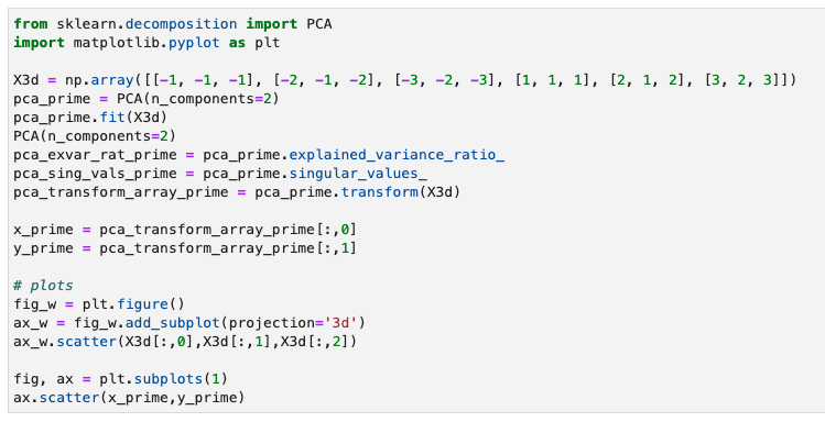
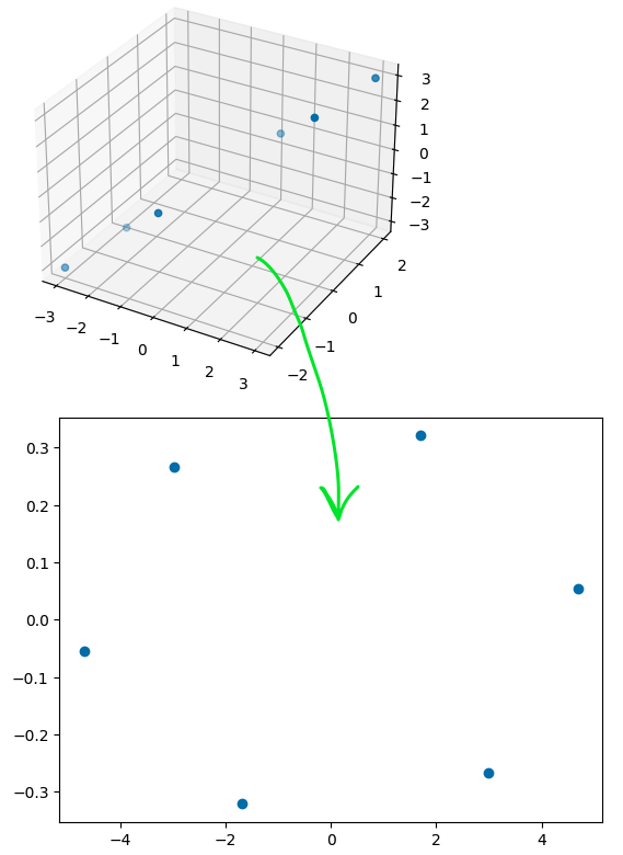
This might look arbitrary, as though the PCA transform function is just putting the points, “wherever,” to make it look nice, but it is applying the transform in a completely predictable way, minimizing variance, so that the reverse would always result in the original array.
So next we’re going to need to iterate through a dataframe to apply comparative sentence analysis across all of our essays. This article goes through some iteration method comparisons.
towardsdatascience.com/heres-the-most…
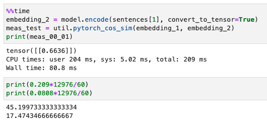
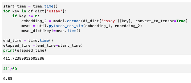
During one iteration we have to find a sentence embedding and find the cosine similarity with Pytorch. Looking at the time it takes for one operation and multiplying by 12976 essays we estimate that this should take anywhere from 17 to 45 minutes, based upon the first two essays.
Testing this out in practice on a dict we find that the elapsed time to compare one sentence to 12976 others took about 7 minutes rather than 17, this could have been because some of the, “essays” are significantly shorter than others, as in one sentence.
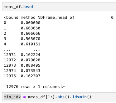
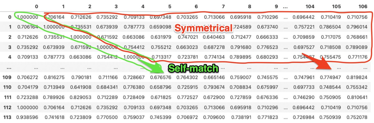
After putting the cosine similarity scores back into a Pandas dataframe and briefly inspecting them, we see distance measurements that are relatively, “far apart,” and “close together” in similarity. We grab the index of the shortest absolute value distance.
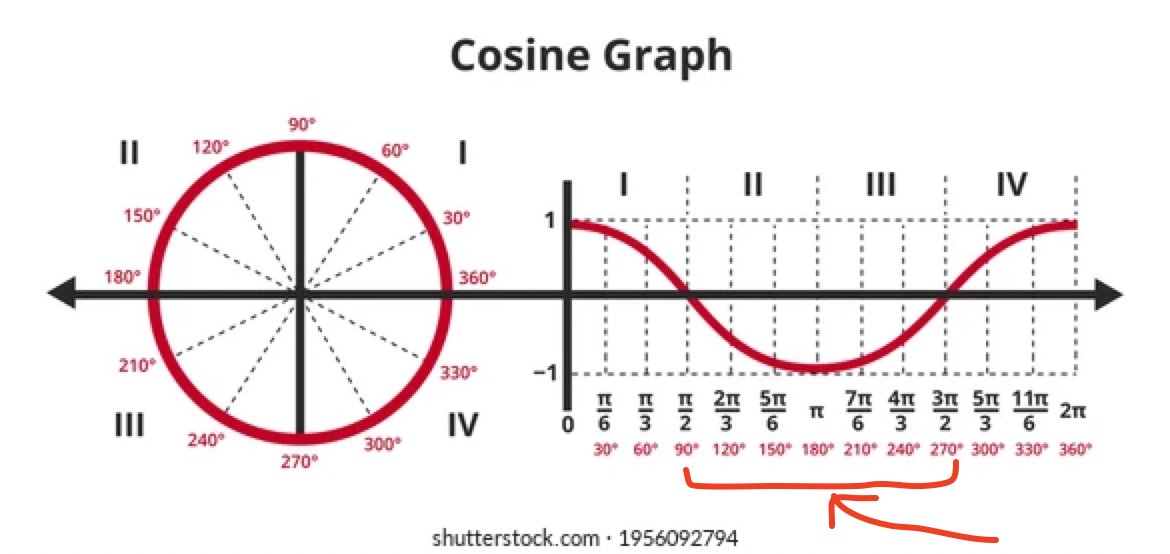
What does cosine similarity mean again, conceptually? It’s basically calculating the, “cosine of the angle” between two vectors.
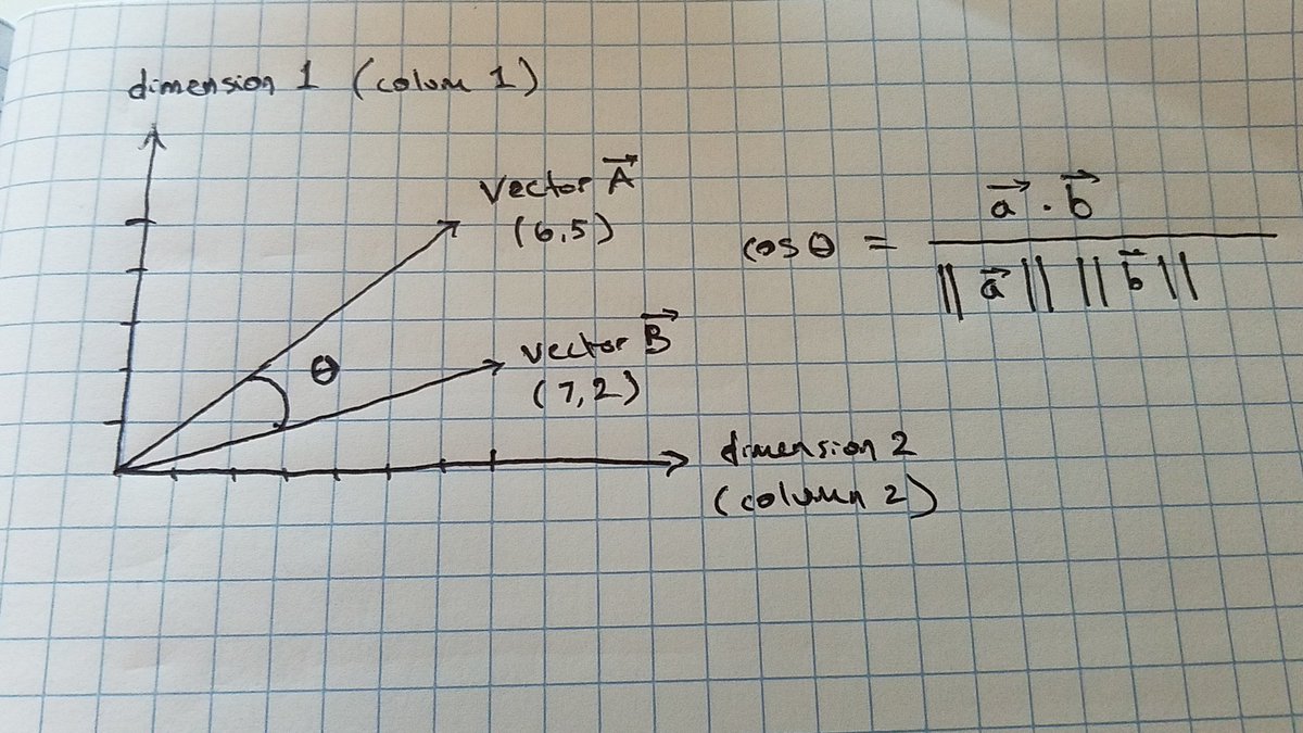
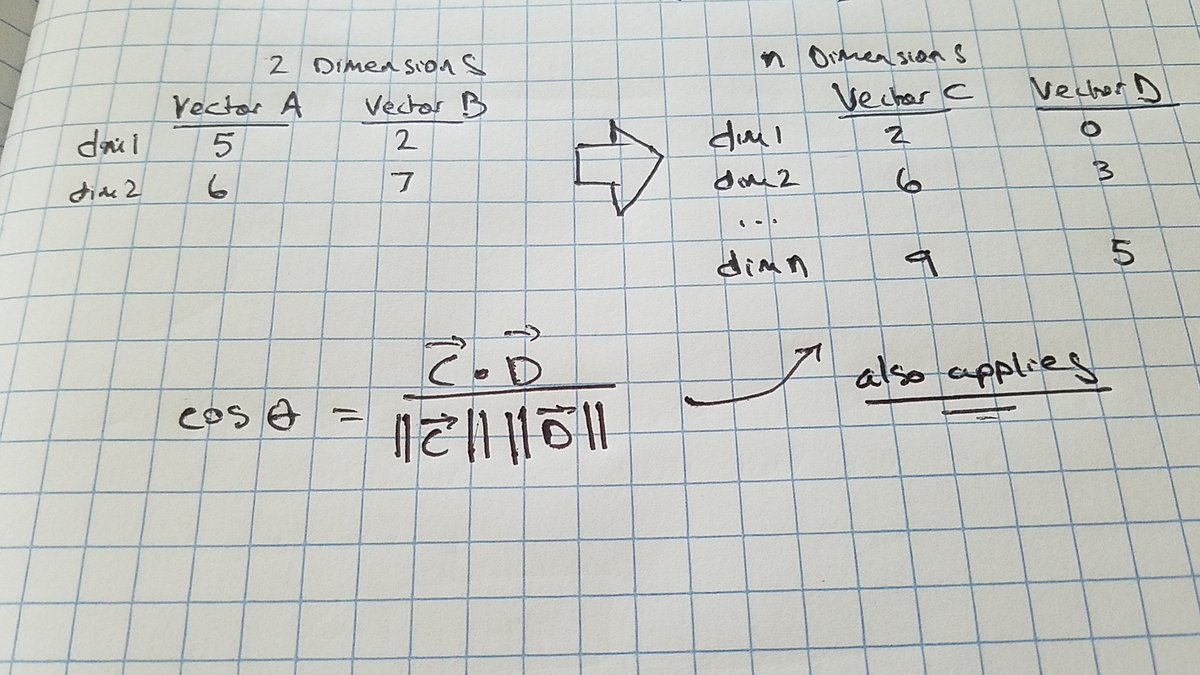
The cosine similarity applies to vectors with an arbitrary number of dimensions, so could be hundreds. These dimensions are word embeddings, so numbered words, parts of speech, fragments, phrases, sentences or however the particular embedding works.
Based upon this, you could have a negative cosine similarity. This is why we take the absolute value of the results, to find the smallest magnitude distance that we can.
So looking at the smallest magnitude (most similar) item first we notice a cosmetic issue, our first essay [0] was enclosed in double straight quotes, so it gets extracted as a string, while essay 6383 was not, so it gets extracted as an object, which means we have to add .item()
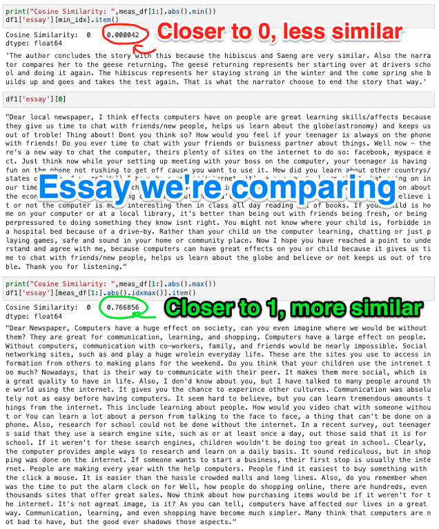
Secondly, we notice that the essay with the smallest cosine value, closest to 0, has nothing to do with the first essay, whereas the cosine similarity value closest to 1, was definitely written using the same prompt as our comparative original essay. Wow! How does this work?
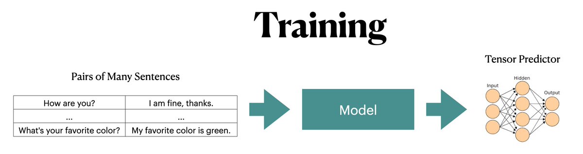
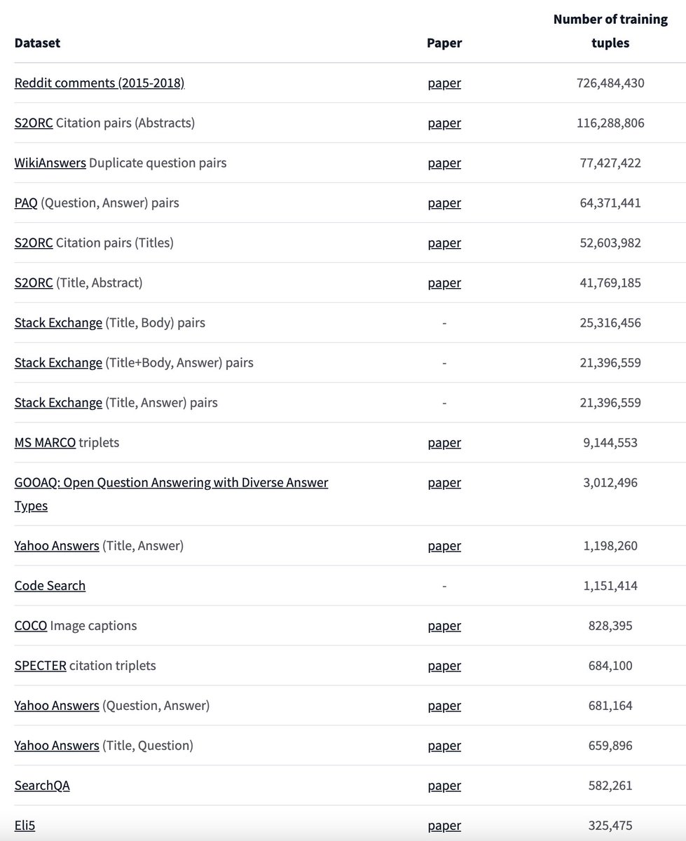
The word embedding model we are using at the base of everything that outputs a tensor score, mpnet-base-v2 was created at a hackathon, where they trained a word embedding model using some special TPU’s, fancy GPU’s which they had access to.
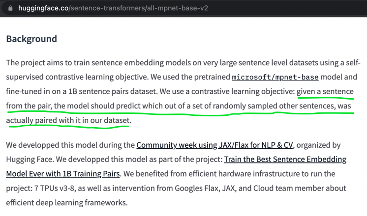
During the hackathon, the training process basically looked like this, they took a billion sentence pairs, trained model that outputs a “filter,” which can be used to create, “tensors,” which are objects that can describe how they relate to other objects in a space.
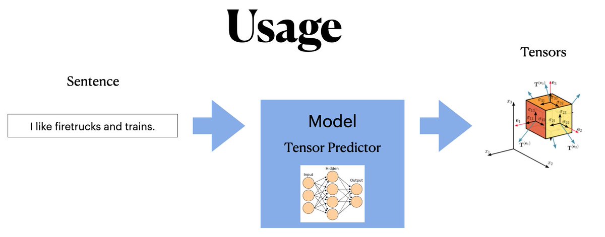
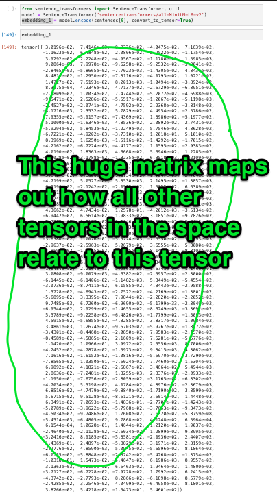
We use this Tensor Predictor Model that they created to make tensors, basically huge matrices, the values of which map out how they relate to all other tensors in a, “space.” This space is defined by all of the total words and sentences found in that original training process.
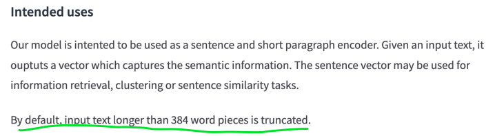
Note, there is a limitation to this Tensor Predictor, it cuts out anything longer than 384 words. But other than that, those tensors describe a position in a space, not a 3d space, but a many-dimension space derived from all of the words used.

Cosine similarity works to compute distances (or angles, really) with whatever number of dimensions, not just two. As long as the original embedding model, the “structure,” was solid, then the cosine similarity is just walking through the front door.
So now that all of this is understood, we can move on to creating a super simple plagiarism detector which works within the limitations of our laptop that we’re working with, which means, basically limiting the number of essays that we’re comparing to one another.
Setting a threshold for cosine similarity from essay[0], we can reduce the total number of essays evaluated. By setting the threshold to, “>0.69” we get about 100 essays to compare, which will take significantly less time for a demonstration.
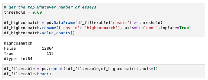
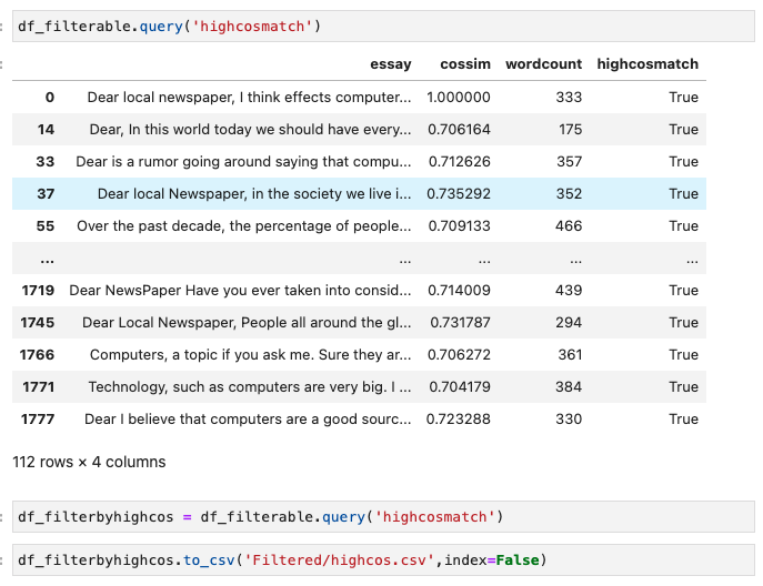
We can create an expanded dataframe which allows us to filter out essays by cosine similarity with booleans, and then we can export this to csv as our temporary database.
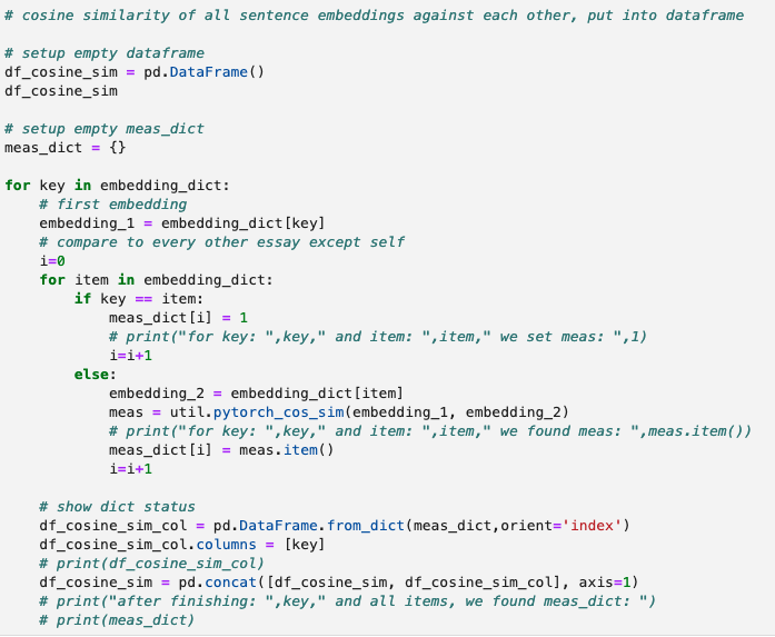
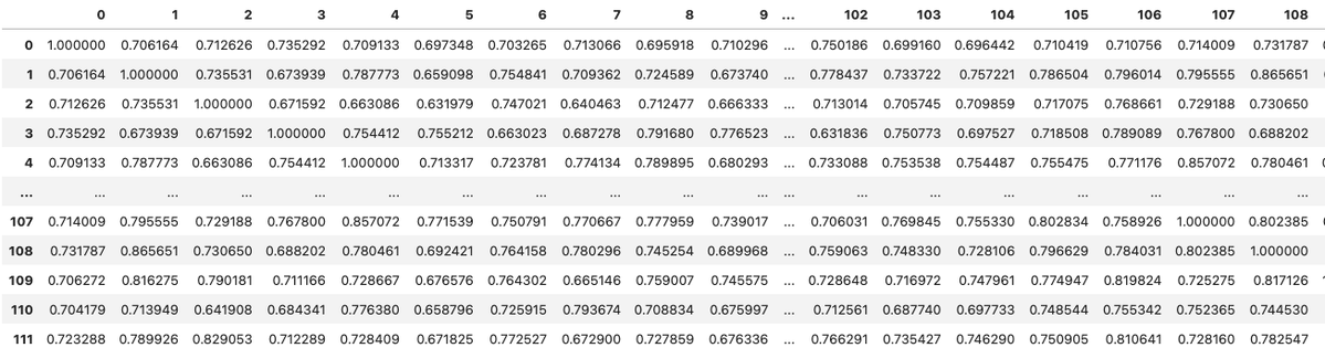
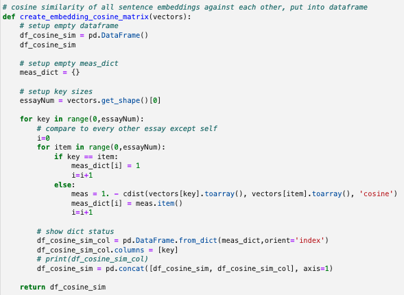
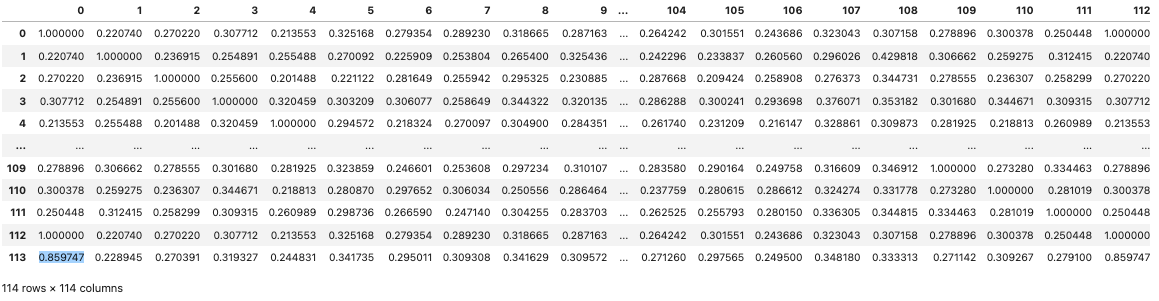
If we want to do PCA and K-Means clustering, we need a big cosine matrix, which we can create by doing nested for loops and comparing embeddings of every single essay with every other single essay, and putting the results into a big matrix.
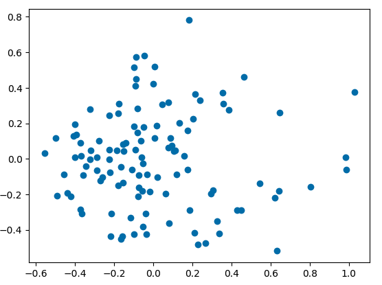
Next we run Principle Components Analysis (PCA) on that matrix to reduce all of the variables down to two, so that it can be plotted on an x-y coordinate system.
Each one of these dots represents an essay, and the distance between the dots represents our having reduced the huge matrix of cosine similarity down once again into two variables which represent the difference of the essays from one another in 2 dimensional space.
We can then run k-means clustering, arbitrarily assigning 3 clusters, to take a look at what different, “topic” areas might be. These clusters look pretty arbitrary, particularly the yellow and purple.
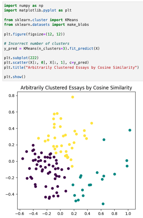
That’s something to keep in mind whenever you do clustering, it always will yield a result, however that result may not mean anything.
But for the purposes of plagiarism detection, maybe we could go in and manually review these essay clusters which are really close to one another - it would be interesting to think about what might have made them fall so close together in our mathematical rendering.
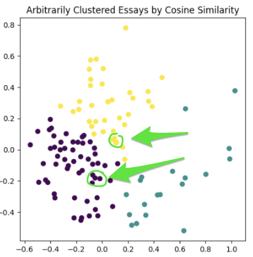
Of course another way to inspect for possible plagiarism could be to just go back a step and look at pairings which had really high cosine similarity, and also think about what it may have been that made these essay pairs so similar from a modeling perspective.
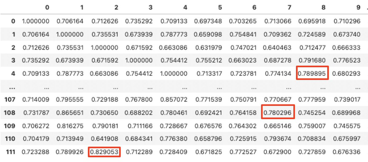
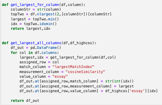
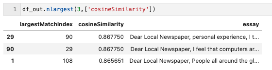
We created a couple functions to operate on our cosine similarity dataframe (df) and the filtered list of high cosine measurements (df_highcos) and spit out a list of the largest cosine similarity matches for every one of our top 112 essays.
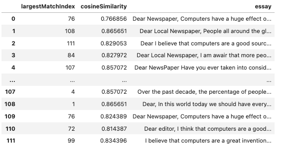
From that we can reduce it down further and do a visual inspection of the top few. We’re showing here that essay 29 and 90 are the highest matches against each other, with 1 and 108 coming in second.
Looking at the two essays against each other, we can make some educated guesses as to perhaps some of the reasons why these essays were found to be mathematically similar, perhaps just based upon words used and nothing else.
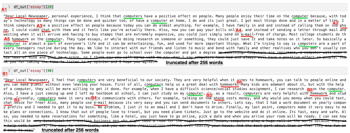
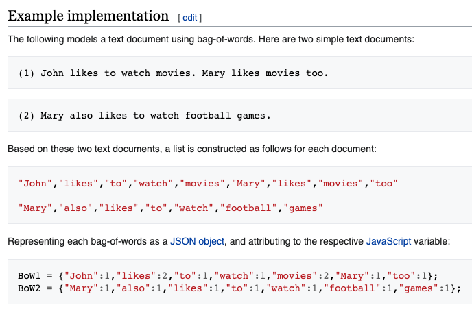
Just looking at words in common assumes a, “Bag of Words,” which assumes that the underlying model was simple a distribution of word counts. (from wikipedia):
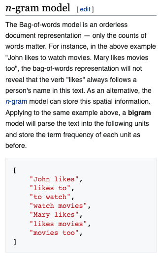
The next step up from, “Bag of Words,” is “n-gram,” which looks at distribution of small phrases, perhaps 2, 3 or 4 word common phrases (from wikipedia).
Instead, the basis of how relations between the text are found is via MPNet, a sophisticated language model designed by researchers and released in 2020.
huggingface.co/docs/transform…
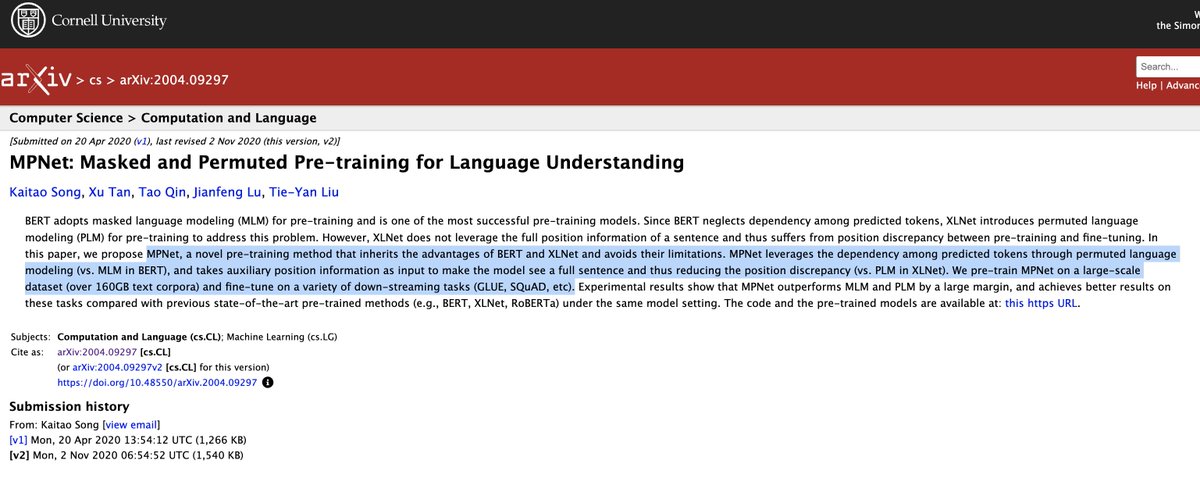
What MPNET does, according to this blog post, is it combines masking of words, something that BERT does, and permutations of words, something that XLNet does. The results of combining the methods are allegedly superior.
microsoft.com/en-us/research…
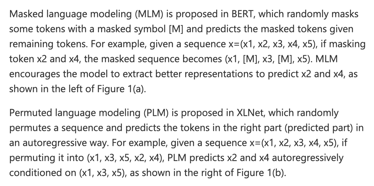
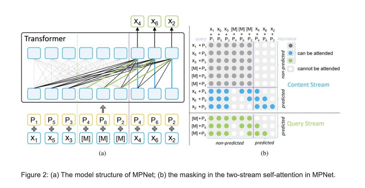
So basically, if you have a sentence (sequence) among many like, [“i”,”like”,”dogs”] it may randomly either mask or permute every few sentences into, [“MASK”,”like”,”dogs”] or [“like”,”dogs”,”i”]
So let’s take a step back - what does, “Training a Language Model,” even mean from a high level and how does a trained language model get used to create one of our, “Tensors,” - e.g., sentence predictions?
What we’ve been talking about with BERT, MPNet, or GPT-3 is essentially generating a statistical understanding of sequences of words based upon many terabytes of text. This is known as training a General Pretrained Transformer Model.
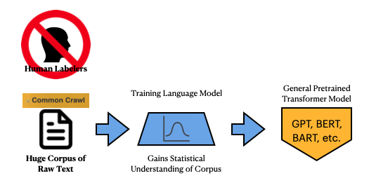
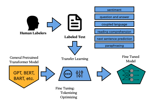
Once these general models get pretrained, they can then be pulled down as an open source model and used to fine-tune a model. So basically the output is a Fine-Tuned Model, derived from that original General Pretrained Model, which can be used for an application.
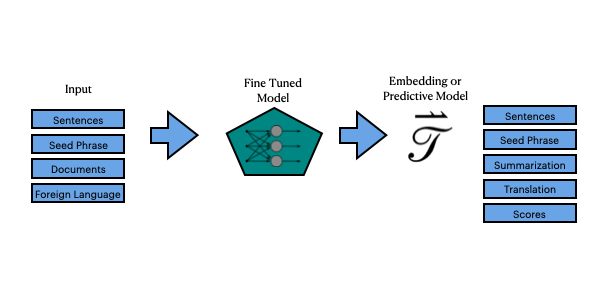
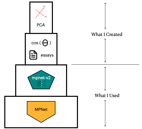
All we have done so far is taken an existing Fine-Tuned Model, mpnet-base-v2, and used it to create tensors, (our scoring method to measure similarity).
huggingface.co/sentence-trans…
So while our original, “Statistical Understanding of Language,” was from the General Pretrained Model known as MPNet, and uses some tricks to create a more accurate model of sequences of sentences, which results in better tokenization and sequencing…
The fine-tuned model we used, mpnet-base-v2, took MPNet and created a model that matches sentences, based upon another database of matched sentences. Those matched sentences were from Reddit, Yahoo Answers, StackExchange, etc. etc.
So our entire plagiarism similarity detection model is really built upon a foundation of two different models, one general and one purpose-built. I simply added some data to analyze and applied cosine similarity / PCA on the output of those models used.
So how can we know whether this plagiarism detection tech stack can even…you know…detect route plagiarism? Well, we have to feed in some purposely plagiarized essays and compare the score of those essays against our already detected, “very similar,” essays.
By the way, you can look at the MPNet tokenizer right here as a JSON file:
huggingface.co/microsoft/mpne…

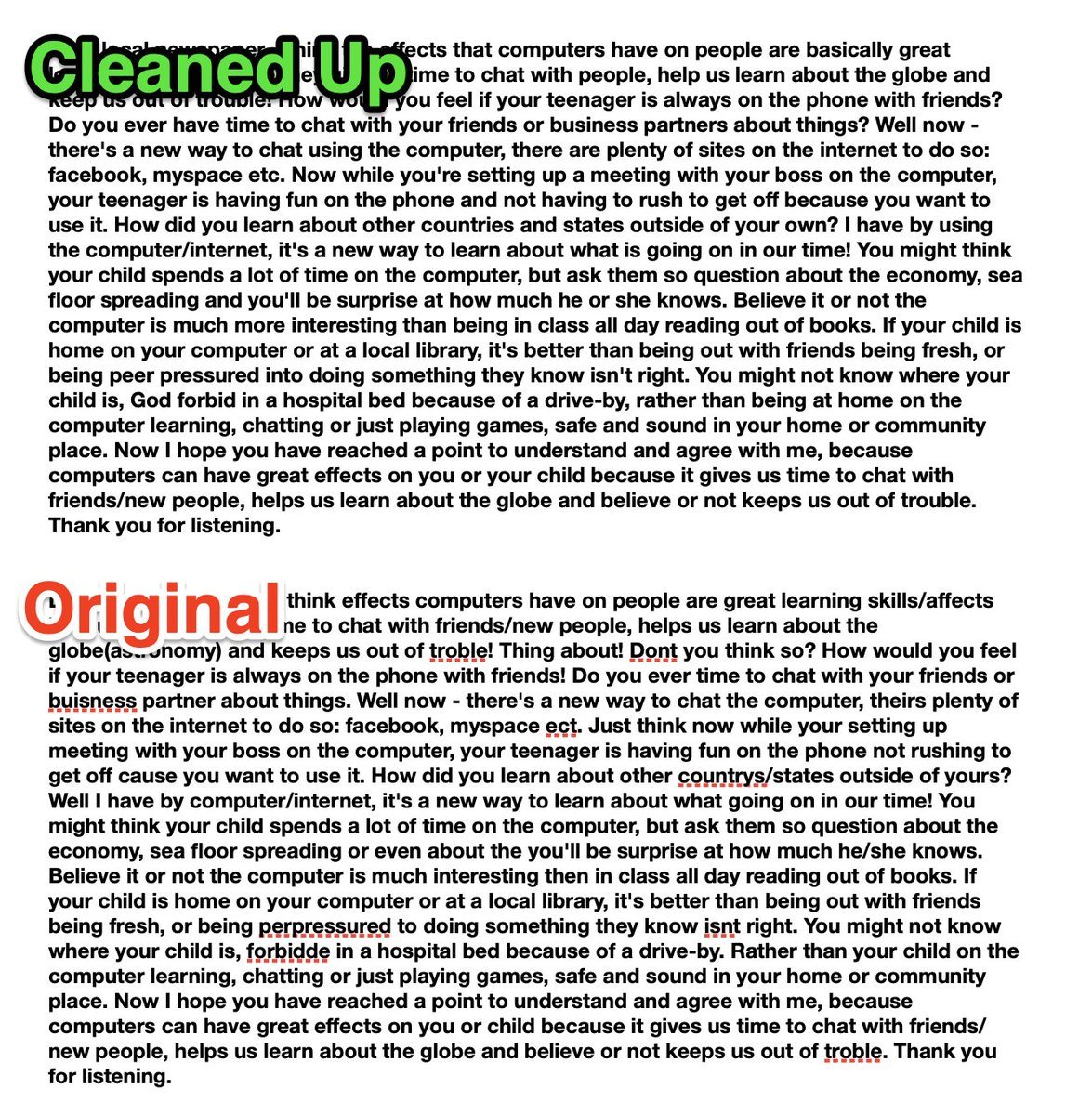
So we threw a couple new essays into the CSV, one completely rote-copied version of essay[0], and another where we attempted to clean up some of the atrocious writing, but left the essay in as much of the original as possible, as shown here:
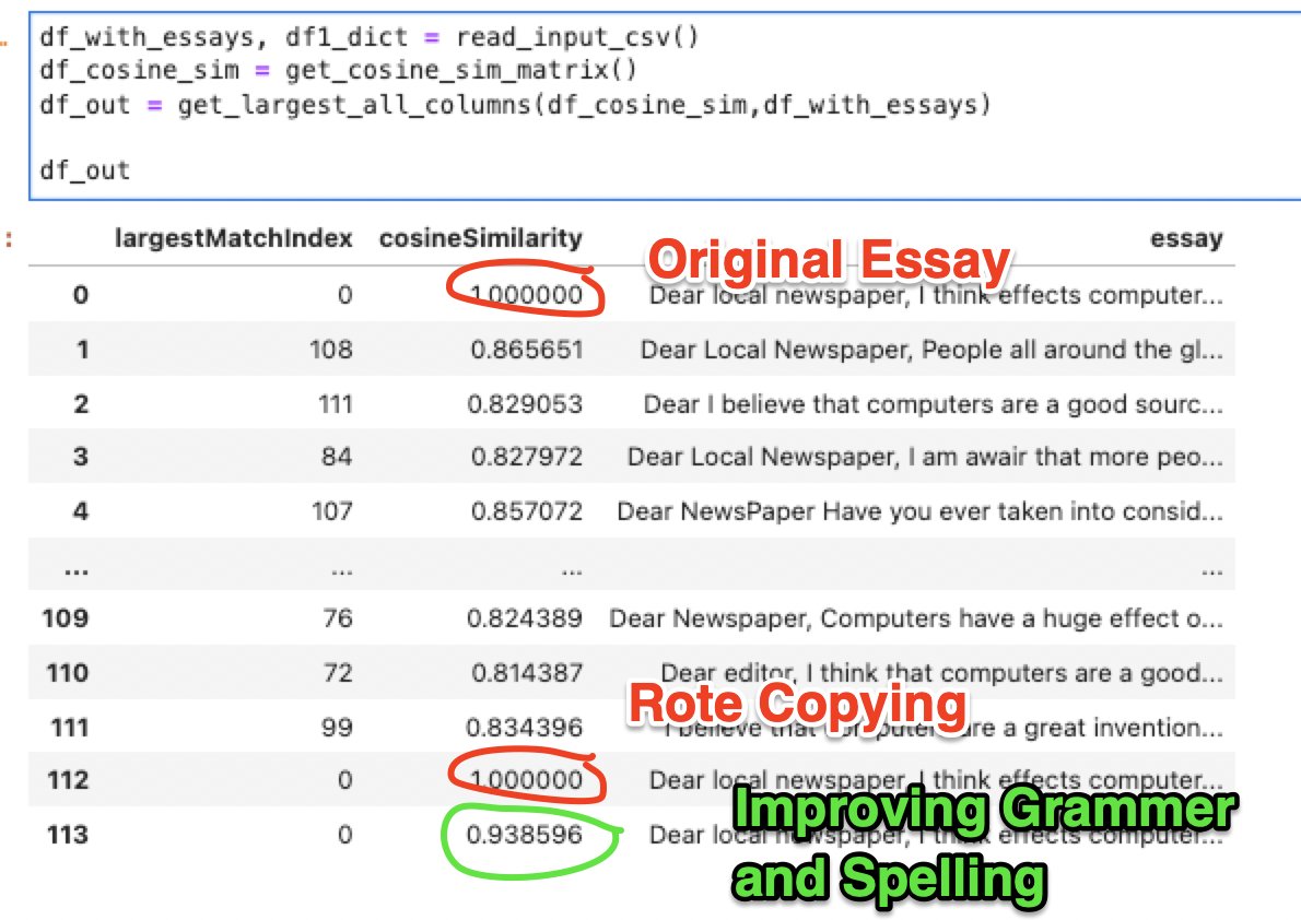
We turned much of the previous work into functions, and input the two versions of essay[0] mentioned above, and our rudimentary plagiarism detector report measured a 1 on the rote copy, and a ~0.939 on the reworded version.
So next it would be interesting to do some statistics on the calculated cosine similarities, and to see what the distribution curve looked like, and how much outside the variance, median and average our, “improved grammar” version lied to see if this could be repeatable.
It would also be interesting to compare this finding to perhaps some other fine-tuned language models and see if we come up with different results. Finally if we have time it might be nice to put this detector into a command-line tool.
Here’s a filtered set of results of a bunch of different ready-made fine-tuned models, specifically for sentence similarity applications.
huggingface.co/models?languag…
There are a number of plagiarism checker tutorials on YouTube:
youtube.com/results?search…

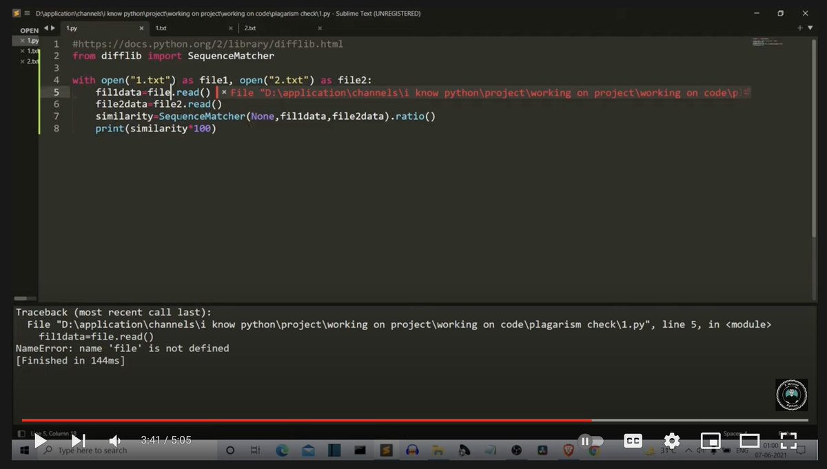
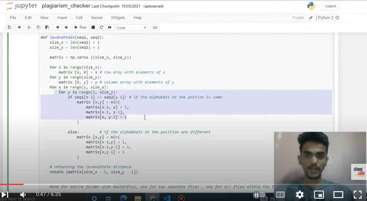
What’s interesting is that none of these seem to make use of Pandas, although some do make use of Numpy, and they don’t seem to be aware of the concept of Transformers. Some seem to be more in-line with being computer science algorithm exercises.
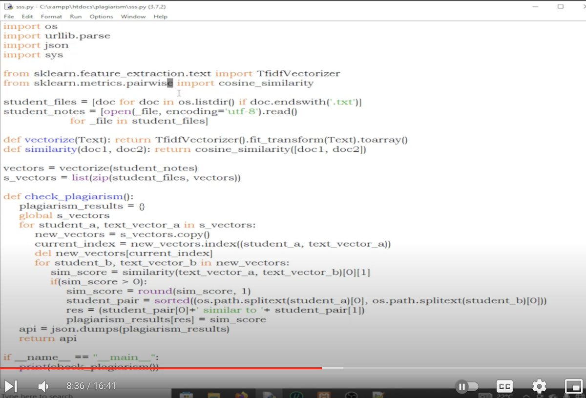
Here’s a nice tutorial put together using scikit-learn TfidfVectorizer and cosine similarity checker.
kalebujordan.dev/how-to-detect-…
Before using another method to create a cosine similarity matrix, it’s important to get more of a statistical description of our mpnet-v2 derived cosine similarity matrix. We can use this to help compare and contrast performance.
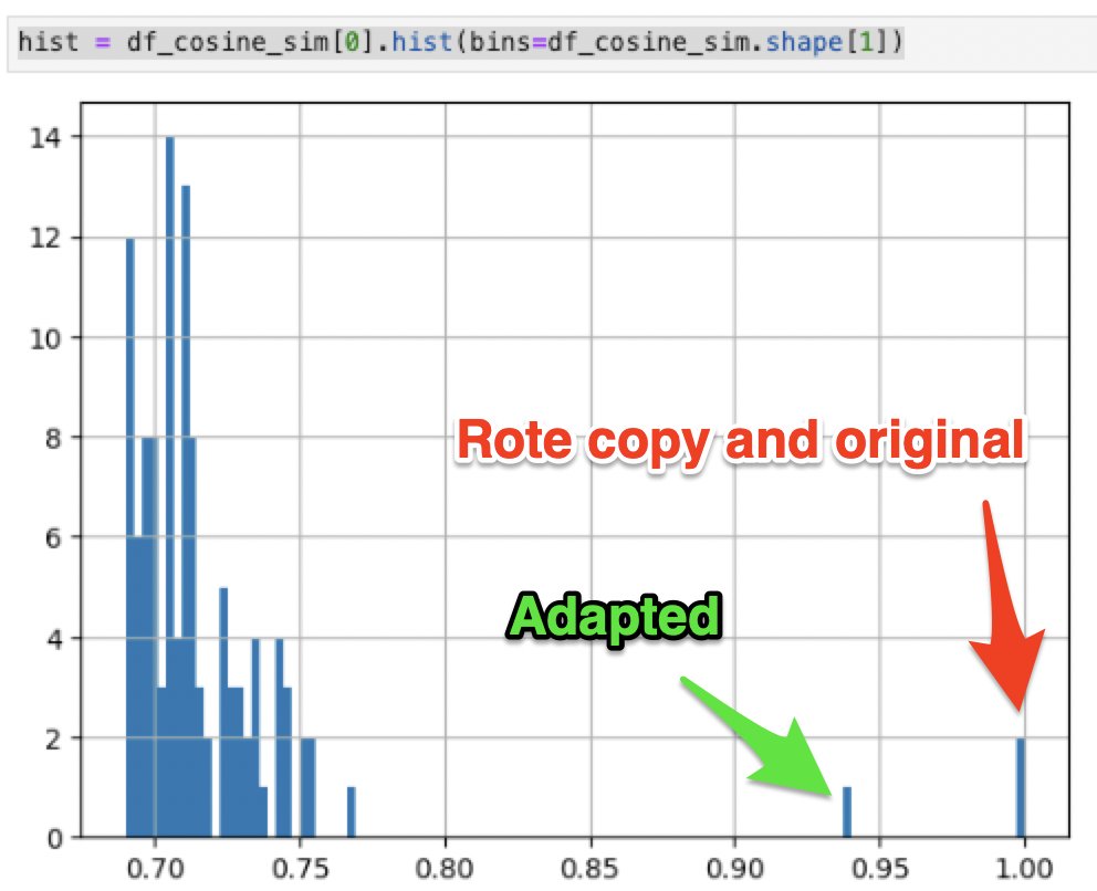
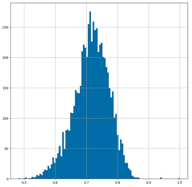
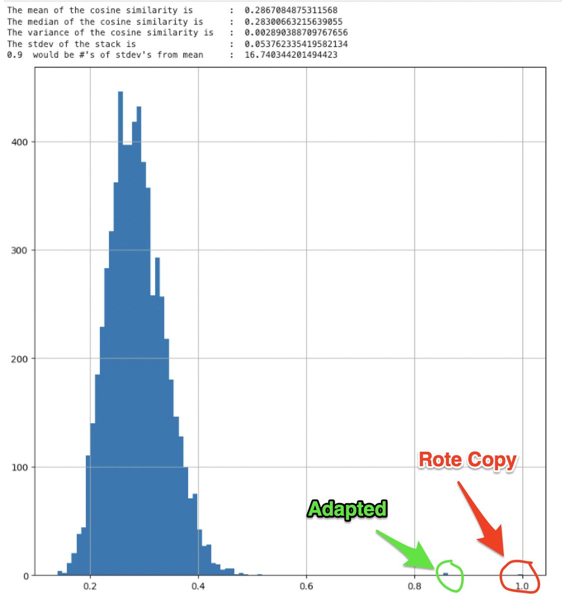
Looking at the histogram for essay[0], we see that we get one match for itself and one for the rote copy, as well as a match that stands fairly fair away for the adapted copy.
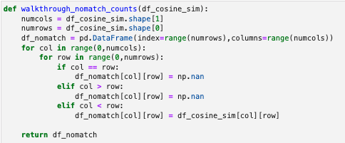
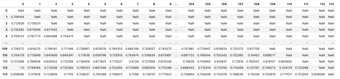
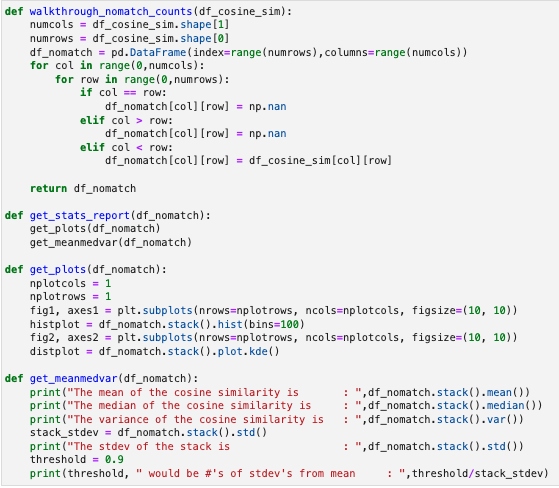
So to eliminate the duplicates we did a walkthrough of the dataframe, replacing said duplicates and self-matches with np.nan values, which resulted in the dataframe shown.
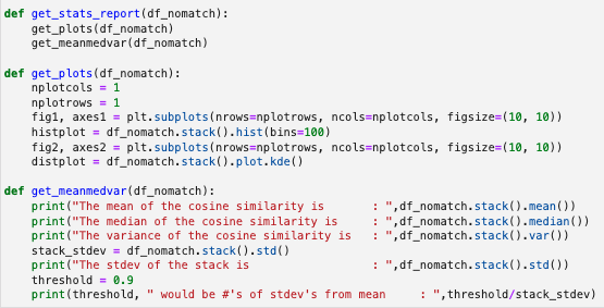
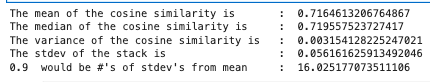
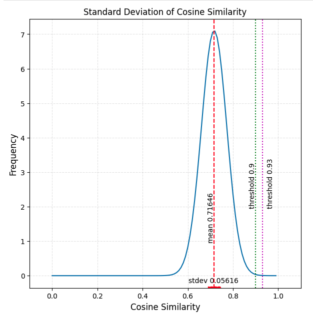
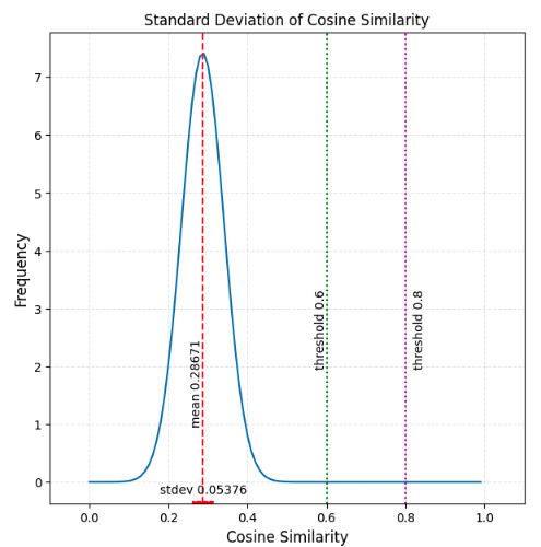
We were then able to get a basic stats report as well as a histogram and a probability density function (PDF).
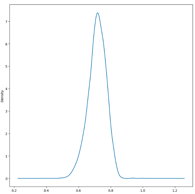
If we convert the PDF to a Standard Normal PDF, applying the law of large numbers and assuming many many texts, you can see that there is a small possibility of false positives (or true positives) under the curve between a threshold of 0.9 and 0.95.
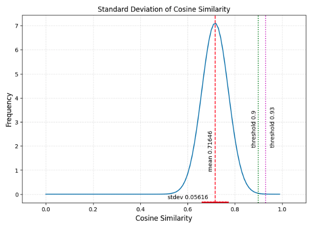
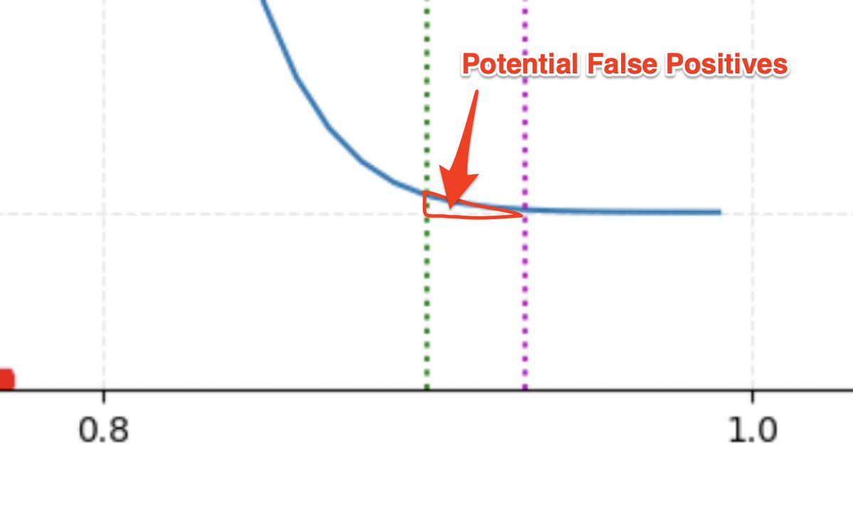
Keep in mind that our original reworded-plagiarized text measured at about 0.93, so 0.95 would not have been sensitive enough, but 0.90 would have been sensitive enough to be able to capture that type of plagiarism.
Here’s a corrected version of the chart above. Note that the stdev is about half of what was shown above, and the upper threshold we are showing is 0.93, not 0.95.
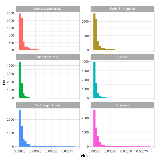
So what if we compare this to another method, TF-IDF (term frequency - inverse document frequency)? This basically compares the frequency of terms used in a document vs. many others in a corpus. Here’s an example showing TF-IDF of Jane Austin novels.
tidytextmining.com/tfidf.html
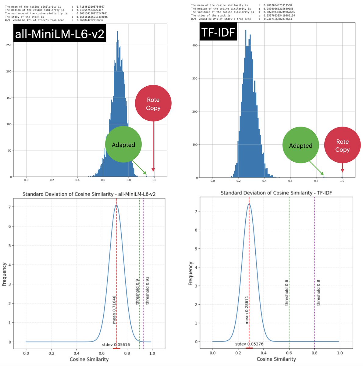
So I built my own TF-IDF using scikit-learn and then built a cosine similarity matrix using scipy. I then cleaned up the cosine matrix and did some stats on it to get a comparison to our fine-tuned, all-MiniLM-L6-v2 transformer model.
The results were staggering. Now the mean of the vast majority of all documents was way over at 0.287, very far away from the adapted copy, which was now at 0.859747, 11 stdev’s away from the mean as opposed to 3.
Translating this over to a hypothetical generalized model, using the law of large numbers and a Standard Normal curve, we have much more breathing room to set thresholds for plagiarism alarms. Interestingly the stdev for TF-IDF was almost the same as for all-MiniLM-L6-v2.
So if I am to bring this to a conclusion, I would say that for the narrow application of comparing all submitted papers to one another as a corpus, TF-IDF on the surface seems like a better model.
Here are the two models next to each other to give a clearer perspective. Again, for rote and slightly adapted plagiarism detection, the regular statistical-based TF-IDF model gives much more leeway.
New questions arise here: 1. Are there any examples we can find of a fine-tuned transformer model or other NN model that can outperform TF-IDF in within-corpus plagiarism detection? 2. What happens to both models if we adapt the essay further? 3. How much time did each take?
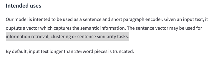
To be fair, SBERT classifies all-MiniLM-L6-v2 as general purpose, which means it’s designed for clustering, information retrieval and sentence similarity. It may be a, “jack of three trades, master of none,” type scenario going on.
sbert.net/docs/pretraine…
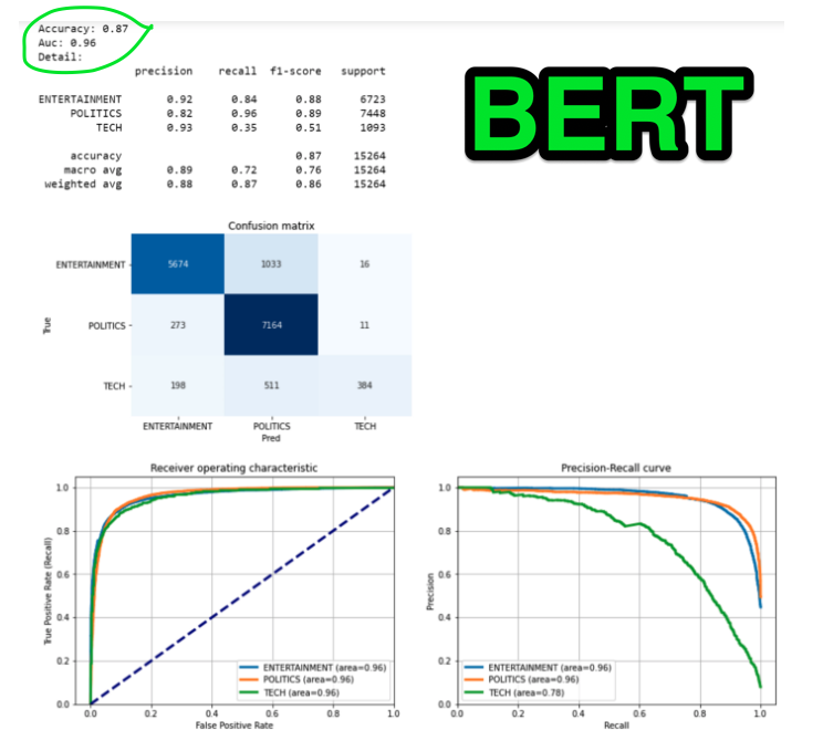
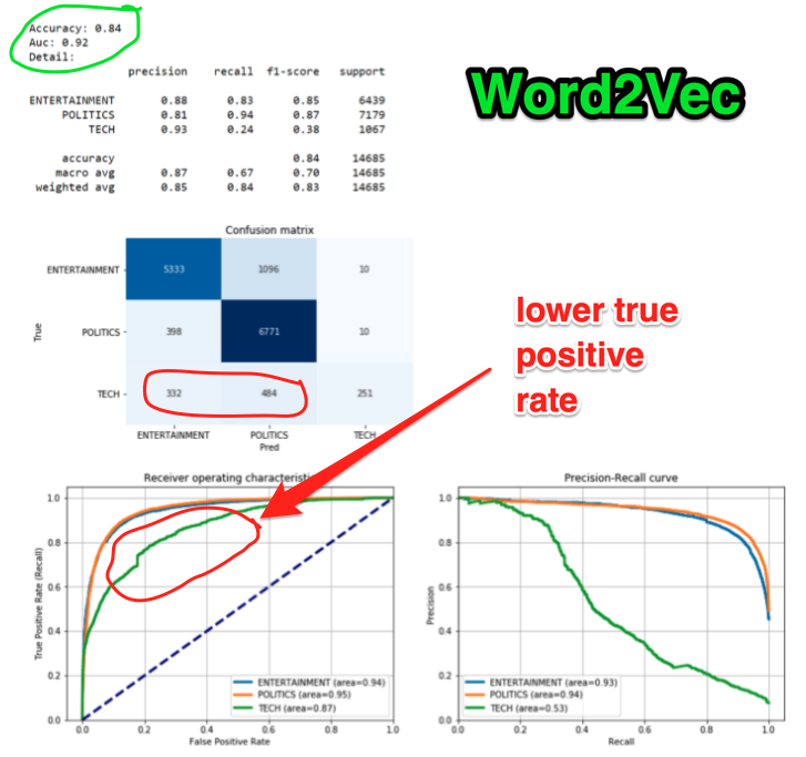
This blog post seems to demonstrate that a BERT model was able to classify articles better than TF-IDF and another bag-of-words type method, Word2Vec.
towardsdatascience.com/text-classific…
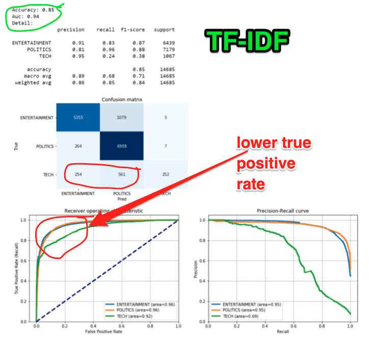
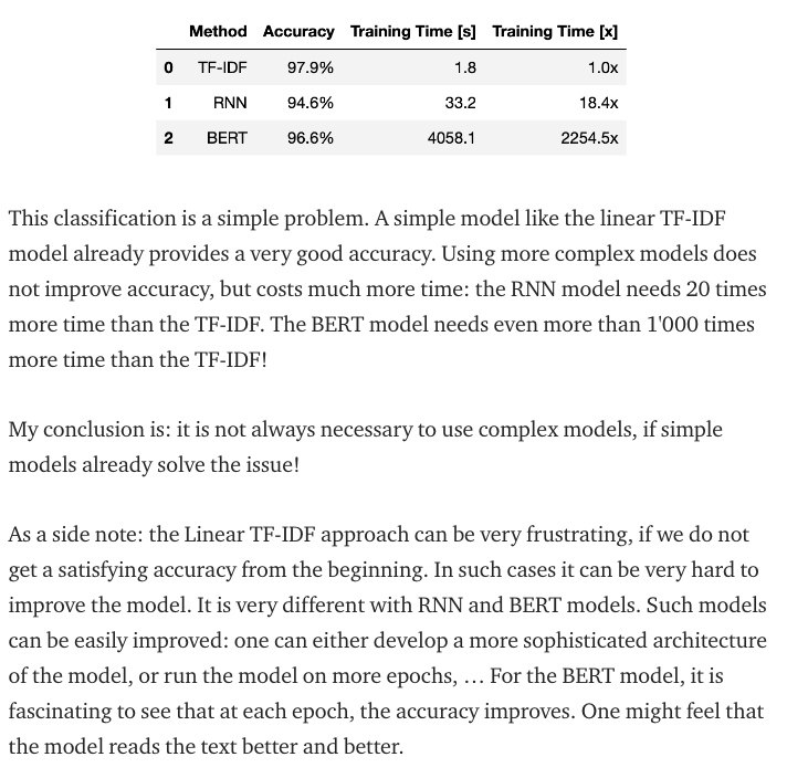
However, this blog post seems to show that with his analysis, TF-IDF was able to perform better for document classification.
datagraphi.com/blog/post/2021…
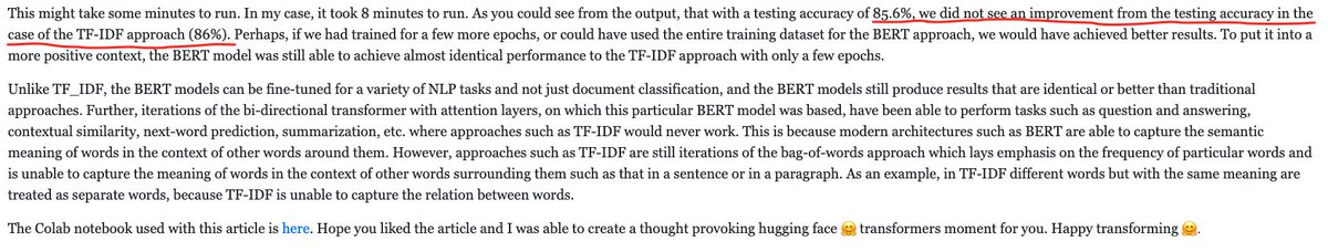
Yet another blog post concludes that TF-IDF is superior for document classification. However it is noted that BERT can be improved over time, whereas TF-IDF is fixed.
medium.com/@claude.feldge…
So why even use a transformer model? Well, it comes down to the application and size of data you are working with. With TF-IDF you are constrained to using an increasingly large matrix as your corpus grows.
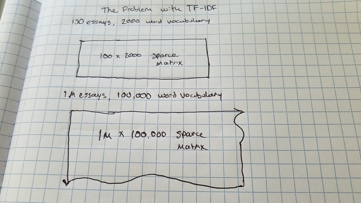
So basically what this means is, if we are using a bag-of-words model, and we’re applying it against very large datasets, huge amounts of text across the web, then we will end up slowing down downstream applications.
Whereas transformers use something called a, “dense model,” so while the accuracy might be less, those, “vectors” (tensors) representing paragraphs will only ever be so large, in the case of all-MiniLM-L6-v2, they will only ever be 384 dimensions.
This means that transformers can hold, “knowledge,” about vocabulary and how sentences should be structured based upon massive datasets, meaning in both the Generalized Pretrained Model (gigantic), and the Fine Tuned Model (huge but less gigantic).

This is something key that I don’t see covered in these performance comparison blogposts: transformers map reduce: they cast a wider net over a much larger dataset which enables one to build an application that will execute in a reasonable timeframe with that dataset.
Here is how I see a plagiarism detector for a very large corpus of documents potentially being architectured, presuming there are budgetary and time constraints.
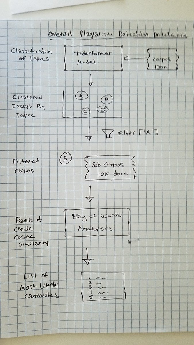
Classifying an article by topic using something like BERT could help map reduce a massive corpus into smaller subsets, which would have more reasonable sparse matrix sizes, allowing TF-IDF or other statistical methods to be performed within that subset.
Share